Deferred Harvest on Smallholder Lands v1.0

1.0

Introduction

This Module provides the requirements and procedures for the calculation of net carbon dioxide equivalent (CO₂e) removal from the atmosphere through improved forest management (IFM) practices implemented by small forest landowners.

Small forest landowners represent a significant portion of the United States' forest ownership, controlling approximately 36% of total forestland¹. These landowners can substantially contribute to climate change mitigation through IFM practices. However, small landowners face disproportionate barriers to participating in carbon markets due to high transaction costs, complex verification requirements, and limited technical resources.

This Module addresses these systemic barriers by establishing a comprehensive approach to crediting specifically designed for small landowner participation in carbon markets with a design that incentivizes improved ecological and economic outcomes for small private landowners while leveraging technological innovations to reduce participation barriers. The Module focuses on deferred timber harvest strategies that allow forests to accumulate additional carbon beyond baseline management scenarios while maintaining the economic viability of forest ownership for participating landowners.

Carbon accumulation is quantified through a dynamic matching baseline approach that compares project forests to similar reference forests within the same region, accounting for variations in forest type, management history, and site conditions. This Module ensures accurate quantification of additional carbon benefits while reducing the technical burden on individual landowners through continuous change detection owned by Isometric and the Project Proponent. The Module employs advanced remote sensing technology, including LiDAR-enhanced-enhanced forest inventories, to monitor carbon accumulation with high precision across multiple small properties while maintaining rigorous standards for measurement, reporting, and verification and reduced field-based verification costs.

To ensure ecological integrity and biodiversity conservation, this Module requires a high proportion of native species composition within project areas and prohibits enrollment of plantation forests and monoculture systems. The Module includes provisions for invasive species management to enhance ecosystem function and resilience throughout the Crediting Period.

Further, this Module ensures the economic sustainability of project activities for participating landowners through guaranteed revenue sharing arrangements, with landowners receiving a large share of Credit revenue. Contract durations are established based on the biological rotation ages specific to forest types, with a conservative 50-year net-impact deduction to ensure meaningful carbon storage duration.

This Module accounts for the quantification of the gross amount of CO₂e removed via enhanced carbon storage in forest biomass, as well as all cradle-to-grave life-cycle Greenhouse Gas (GHG) emissions associated with the implementation process. This Module is developed to adhere to the requirements of ISO 14064-2: 2019 – Greenhouse Gasses – Part 2: Specification with guidance at the Project level for quantification, monitoring, and reporting of greenhouse gas emission reductions or removal enhancements.

The Module ensures:

Consistent, accurate procedures are used to measure and monitor forest carbon accumulation through standardized methodologies appropriate for small landowner implementation;
All net CO₂e removal claims are verified through robust field work and LiDAR-enhanced monitoring systems and third-party validation;
Forest management practices maintain ecological integrity through native species requirements and biodiversity conservation measures;
Removals are additional through the use of dynamic matching baselines that account for regional management practices and other guardrails set forth in the Isometric Standard;
Dynamic baseline methodologies provide accurate quantification of additional carbon benefits through regional reference comparisons;
Comprehensive risk management through buffer pools and optional insurance mechanisms protects against potential reversals while ensuring transparent Credit delivery;
Economic viability for small landowners through guaranteed revenue sharing and appropriate contract terms; and
Technology-enabled monitoring reduces transaction costs while maintaining high standards for carbon accounting and environmental integrity.

Throughout this Module, the use of "must" indicates a requirement, whereas "should" indicates a recommendation.

2.0

Sources and Reference Standards & Methodologies

This Module relies on and is intended to be compliant with the following standards and protocols:

The Isometric Standard
Improved Forest Management v1.0, Isometric
ISO 14064-2: 2019 - Greenhouse Gases - Part 2: Specification with guidance at the project level for quantification, monitoring, and reporting of greenhouse gas emission reductions or removal enhancements

Additional reference standards that inform the requirements and overall practices incorporated in this Module include:

ISO 14064-3: 2019 - Greenhouse Gases - Part 3: Specification with Guidance for the verification and validation of greenhouse gas statements
ISO 14040: 2006 - Environmental Management - Lifecycle Assessment - Principles & Framework
ISO 14044: 2006 - Environmental Management - Lifecycle Assessment - Requirements & Guidelines

Additional principles that were considered in the development of this Module and aligned with, where feasible, include:

The Core Carbon Principles of The Integrity Council for the Voluntary Carbon Market, v1.1, ICVCM, 2024
Criteria for High-Quality Carbon Dioxide Removal, Carbon Direct & Microsoft, 2025

3.0

Future Versions

This Module was developed based on the current state of the art, publicly available science regarding IFM activities and long-term monitoring of forest carbon projects. This Module aims to be scientifically stringent and robust. We recognize that some requirements may exceed the status quo in the market and that there are numerous opportunities to improve the rigor of this Module as new approaches and techniques enter the Voluntary Carbon Market.

Additionally, this Module will be reviewed when there is an update to published scientific literature, government policies, or legal requirements which would affect net CO₂e removal quantification or the monitoring guidelines outlined in this Module, or at a minimum of every 2 years.

4.0

Applicability

In addition to the requirements outlined in Section 4 of the Improved Forest Management Protocol, Projects are subject to the following applicability requirements, which must be demonstrated in the Project Design Document.

4.1

Viability of the Project and Determination of the Project Area

In order to maintain ecological integrity and ecosystem function, demonstrate additionality, and ensure trust and transparency, it is incumbent upon Projects to adhere to the requirements below, which must be demonstrated and reported in the Project Design Document.

4.1.1

Land Enrollment and Parcel Classes

Given the nature of this Module, it is anticipated that a Project, facilitated by the Project Proponent, may enroll many smallholder landowners within a Project. To ensure accurate carbon sequestration claims and facilitate Validation and Verification, this Module requires that a Project be registered for a singular or grouped site(s) — sets of land parcels subject to similar bioclimatic, regulatory, and geographic conditions.

Sites must consist of land parcels — discrete areas of land as defined by town, county, or regional tax maps. Contiguous sites or sites within 10 kilometers of each other may be grouped into a single site. Large, discontinuous sites more than 10 kilometers apart from one another must be enrolled as separate sites. Each site within a Project must independently meet all eligibility criteria. Carbon quantification, as set out in Section 8.1, will be calculated at the site level. The Project Proponent(s) and landowner(s) must adhere to the following additional requirements for parcel and site enrollment:

All sites must be greater than 10 hectares.
All parcels must have road access.
- Exceptions to this rule apply under extenuating circumstances — such as the presence of an easement or prior commercial harvest history — and can only be claimed after consultation with Isometric.

4.1.1.1

Integrity of Enrolled Land

To ensure the credibility of the climate impact of the Project activities — and Credits — non-additional areas of the Project must be excluded, as set out by various requirements in Section 4.1 of the Improved Forest Management Protocol and Sections 4.1.2 of this Module.

It is vital to the integrity of the Project that no other areas within each parcel may be excluded from project activities. Landowners participating in the Project must enroll all eligible areas of a parcel. This requirement prevents the selective enrollment of areas that are less desirable for harvest. Land can only be excluded for reasons stated within this Module or the Improved Forest Management Protocol, and these excluded areas must meet be documented within the Project Design Document with sufficient justification of the legal, financial, or operational restrictions on harvest and spatially mapped.

4.1.1.2

Parcel Classes

For the purposes of this Module, Parcel Classes will be used for dynamic baselining and carbon quantification — i.e., distributed reference regions used as a point of comparison between behaviors observed in a site and those observed in areas with similar landowners (Figure 1).

Figure 1. Example parcel class distribution within a Project site.

The Project Proponent must generate between 10 and 50 Parcel Classes for the Project by clustering parcels in the ecoregion(s) of the country of the site(s) into groupings with shared socio-economic, topographic, bioclimatic, historical, and structural attributes in relation to the forest. The Project Proponent, where possible, must incorporate the attributes found in Table 1 into its clustering approach.

Table 1. Parcel Classification Clustering Attributes

Cluster Category	Variable	Potential Datasets
Economic	Land value	Nolte, et. al. 2020; Local property tax assessments; Real estate market data
	Building Presence	Cadastral records; Zoning data; Building permits database
	Building footprint area	High-resolution satellite imagery; Municipal building databases; OpenStreetMap building footprints
	Distance to highways	OpenStreetMap road networks; National highway databases; Transportation department GIS data
	Distances to mills	Forest industry facility databases; Manufacturing facility registries; Economic census data
	Distances to urbanized areas	Census urban area boundaries; Land use/land cover datasets; Municipal boundary files
	Distances to urban expansion	Historical land use maps; Urban growth models; Development planning documents
	Parcel size	Cadastral/parcel boundary datasets; Property records; Land registry data
Topographic	Slope	Digital Elevation Models (DEMs); SRTM data; National topographic databases
Topographic	Topographic roughness index	DEM-derived metrics; Terrain analysis from USGS; ASTER Global DEM
Bioclimatic	Index of Productivity (BFI, NPP)	MODIS NPP data; Forest productivity indices; Site index databases
	Precipitation (seasonality and annual average)	WorldClim data; National weather station records; PRISM climate data
	Temperature (seasonality and annual average)	WorldClim temperature data; Climate normals; Meteorological databases
Historical	Time since last commercial forest harvest	Forest management records; Harvest permit databases; Silvicultural treatment histories
Structural	Carbon stock (LiDAR-derived)	Airborne LiDAR surveys; Forest inventory plots; Biomass estimation models
	Merchantable volume (LiDAR-derived)	LiDAR forest metrics; Timber cruising data; Forest inventory databases
	Stem Density (LiDAR-derived)	LiDAR point cloud analysis; Forest stand data; Tree count surveys
	Species groupings	Forest type maps; Vegetation surveys; Species composition databases

4.1.2

Ecological Feasibility of Harvest

Project activities must demonstrate additionality by accounting for site-specific constraints that limit harvesting feasibility under baseline conditions. If ecological and site conditions would render harvesting unlikely under baseline conditions, these areas within the Project Boundary cannot be claimed as additional and must be excluded from the Project Boundary. Soil saturation, permanent water bodies, slope gradients, and proximity to dwellings and other structures create natural and regulatory limitations on small landholder deferred harvesting activities that must be evaluated when determining eligible project areas.

Project Proponents must identify and exclude from Crediting any areas within the Project Boundary where physical or regulatory constraints make harvesting highly unlikely under baseline management scenarios.

4.1.2.1

Soil Drainage Limitations

Historically, harvesting operations in waterlogged soils occurred primarily during periods of prolonged freezing temperatures, which provided ground stability for heavy timber equipment. Climate change has reduced the predictability and duration of these freezing periods, particularly in temperate and polar regions, making winter harvesting increasingly unreliable. Consequently, harvest avoidance in these soil types does not constitute additional management activity beyond what would occur under baseline conditions.

Project Proponents must identify and exclude from Crediting any areas within the Project Boundary with soils classified as "very poorly drained" or "inundated" according to the U.S. Soil Taxonomy classification system, or similarly classified soils in equivalent authoritative sources if a Project occurs outside of the United States of America.

Exceptions to this rule can be made if the Project Proponent demonstrates all requirements in Section 4.1.2.1.1 below.

4.1.2.1.1

Seasonal Operability Exception

Project Proponents may include areas with soils classified as "very poorly drained" or "inundated" within the Project Boundary where evidence demonstrates that baseline harvesting operations remain economically viable despite soil drainage limitations.

Areas with waterlogged soils may be included when the Project Proponent demonstrates:

Baseline harvesting activities in the region commonly occur during predictable seasonal windows when soil conditions permit equipment access, as evidenced by regional timber market data, harvesting permits, or forestry operation records covering a minimum of the prior 10 years;
Specialized harvesting equipment or techniques (such as winter harvesting, low ground-pressure machinery, or helicopter logging) are established practice in the region for similar soil conditions, demonstrated through equipment rental availability, contractor specialization, or documented use in comparable forest stands; and
The proposed IFM activities constitute a measurable departure from baseline management that would otherwise occur despite drainage constraints.

To include these areas, the Project must demonstrate additionality of these waterlogged soils through financial analysis showing that baseline harvesting remains economically feasible despite drainage-related operational constraints, and that the carbon revenue represents a necessary incentive for the proposed management changes.

4.1.2.2

Proximity to Water Bodies

Project Proponents must identify and exclude from Crediting any areas within the Project Boundary that fall within management buffers around permanent water bodies as defined by applicable governmental regulations or voluntary Best Management Practices (see Appendix C of the Improved Forest Management Protocol).

Project Proponents must provide documentation of applicable governmental regulations and BMPs governing management buffers around water bodies, along with mapping of permanent water bodies and associated buffer zones within the Project Boundary.

4.1.2.3

Geographical Constraints

Project Proponents must provide evidence of common harvesting practices and equipment availability within the relevant wood basket to demonstrate whether steep-slope operations are feasible under baseline management scenarios. This evidence must include a spatially-explicit topographic analysis of slope gradients within the Project Boundary and a regional assessment of harvesting capabilities on steep terrain.

Project Proponents must document the selection of the relevant wood basket, and should ascertain the relevant wood basket by examining governmental, regulatory, or industry databases or identifying the regional catchment of the timber product(s) of their harvest.

Project Proponents must exclude from crediting calculations areas with sustained slopes exceeding 30% over 30 meters in regions where specialized steep-slope harvesting equipment is not commonly deployed.

The U.S. Forest Service has found that harvest equipment encounters significant limitations on slopes of 25% to 35%, with severe constraints on slopes exceeding 35%. Areas with sustained slopes above these thresholds represent natural barriers to conventional harvesting operations.

4.1.2.4

Proximity to Dwellings and Other Structures

Research on non-industrial private forest owner preferences demonstrates that the majority of forest owners will not permit harvesting activities in the immediate vicinity of residential dwellings and other permanent structures². Additionally, regulations or BMPs may prohibit harvesting within a certain proximity of built structures.

Project Proponents must exclude from crediting calculations any areas within 50 feet of permanent structures, or within larger buffers if required by applicable regulations or BMPs (see Appendix C of the Improved Forest Management Protocol).

To meet this requirement, Project Proponents must include a spatially-explicit vector-based map of all permanent structures within and adjacent to the Project Boundary, along with documentation of any applicable governmental buffer requirements which would prohibit harvesting around dwellings and structures.

4.1.3

Merchantable Stocking

Project Proponents must demonstrate that landowners — who have owned the land for more than 5 years — enrolling into the Project do not possess merchantable stocking significantly above the regional average of the Parcel Class. Such stocks of merchantable carbon would indicate a pre-existing intent to conserve or defer harvest in violation of the requirements set out in Section 7.7 Additionality of the Improved Forest Management Protocol.

4.1.3.1

Quantification of Initial Carbon Stock

The Project Proponent must report the initial carbon stock, $M_{AGB}(t_0)$ , of each parcel eligible for enrollment — e.g., initial standing carbon stock value — through a field inventory or with LiDAR according to one of the following Capture & Conversion Modules:

Uses field-based measurements of vegetation species and size taken within sample plots along with allometric equations to quantify biomass.

Uses aerial LiDAR data collected over the Project area and trained models to quantify biomass.

The Project Proponent must then develop and report growth curves for each Parcel Class, which describe the average forest growth trajectory.

Using historical disturbance history over the past 10 years, the Project Proponent must then determine and report the average age (and standard deviation) of harvest within each Parcel Class.

To meet this requirement, the Project Proponent should use the Hansen Global Forest Change Product

The Project Proponent must then document and plot the reported volume or carbon stock of each parcel against the appropriate Parcel Class growth curve, thereby deriving the current stand age of the parcel (Figure 2). If a parcel’s volume or carbon stocking exceeds one standard deviation of that of the average harvest date plus 10 years — to allow for growth into later size-classes — it shall be deemed ineligible for Credits under this Module and removed from the Project.

A growth trajectory of properties within the site’s Parcel Class. (a) The average date and stocking level at harvest within the Parcel Class. (b) Bars surrounding point (a) refer to one standard deviation above and below the average harvest date. (c ) The volume-limit at which sites are not eligible for enrollment, determined by taking one standard deviation above the mean, plus 10 years.

Figure 2. A growth trajectory of properties within the site’s Parcel Class. (a) The average date and stocking level at harvest within the Parcel Class. (b) Bars surrounding point (a) refer to one standard deviation above and below the average harvest date. (c) The volume-limit at which sites are not eligible for enrollment, determined by taking one standard deviation above the mean, plus 10 years.

4.2

Other Requirements

Under deferred harvest, the planting of new trees cannot be the primary method to achieve forest cover. Project Proponents must limit new planting only to fill in gaps in existing patches of degraded forests or to regenerate small areas — less than 0.5 hectares — of otherwise forested land.

The Project Proponent must disclose this planting, as well as the justification for it, within the PDD for initial Validation and subsequent Verifications if any new planting has occurred, and follow all biodiversity requirements as set forth in Section 6.4 of the Improved Forest Management Protocol.

5.0

Project Timelines

5.1

Crediting Period

The length of the Crediting Period of the Project shall be determined by the cumulative temporal maximum of the contract lengths of the enrolled landowner(s) and their site(s) or 20 years, whichever is longer. The contract length for parcels enrolled in the Project is determined by the biological and economic trajectory of the forest stand, and set by an assessment of key forest characteristics measured using this Module’s approved remote sensing technologies, ideally LiDAR. These contracts must meet the requirements set forth in Section 5.1 of the Improved Forest Management Protocol.

Project Proponents must assess three critical parameters — current forest size, estimated biological rotation age, and current stand age — to determine contract lengths for enrolled landowners.

The initial contract length for each enrolled landowner, Contract Lengthlandowner, must be calculated using the following equation that takes these parameters into account:

 $Contract\ Length_{landowner} = (\bar{RA} + RA_{SD} + EP) - CSA$

(Equation 1)

Where:

$\bar{RA}$ is the mean rotation age of the parcel as determined in Section 4.1.3.1
$RA_{SD}$ is the standard deviation of the rotation age of the parcel as determined in Section Section 4.1.3.1 Quantification of Merchantable Stock
$EP$ is the extension period, which is set at $\frac{1}{6}$ of $\bar{RA}$
$CSA$ is the current stand age of the parcel, as determined in Section 4.1.3.1

The Crediting Period will commence either when the Project Proponent commences activities on a site or on the date of the first enrolled landowner contract signature within the Project, with project activities required to commence immediately. No Credits shall be issued for activities that occurred prior to the contract signature date.

Projects seeking to extend the initial Crediting period must demonstrate continued additionality in line with all requirements set forth in this Module, the Improved Forest Management Protocol, and the Isometric Standard.

5.2

Reporting Period

The first Reporting Period shall end at a date set by the Project Proponent and approved by Isometric. This first Reporting Period must occur within 5 years of the initiation of the Crediting Period.

As Projects enroll any additional landowner(s), the parcel(s) from the newly enrolled contract(s), i, must take a deduction of Credits based on the time between the date of enrollment and the end of the Reporting Period according to the following Equation 2:

 $ARPF_i= \frac{Days\space to\space end\space of\space Reporting\space Period}{Total\space Days\space of\space Reporting\space Period}$

(Equation 2)

Where $ARPF_i$ is the Adjusted Reporting Period Factor discount rate applied in Equation 7 to the calculation of CO₂e stored for the parcel(s) under each individual contract, $i$ , weighted to ensure only growth since contract initiation is included in the Credit issuance for the Reporting Period (see Section 8.1).

6.1

Safeguarding of Biodiversity

In addition to the requirements set forth in Section 6.4 of the Improved Forest Management Protocol, Projects must not resemble commercial or monoculture plantations.

In cases where a species naturally grows in monoculture within the Project region or there is scientific evidence for a single dominant species during natural succession, Project Proponents may proceed with monoculture cultivation of this species in consultation with Isometric as outlined in Section 6.4: Safeguarding of Biodiversity.

6.2

Forest Management Activities

While a forest management plan is not required for landowner enrollment into the Project, Project Proponents should work with enrolled landowner(s) to develop parcel- and site-specific plans. Project Proponents should facilitate expert forester consultation with enrolled landowners as part of enrollment into the Project, and disclose any such past or planned activity in the Project Design Document.

Certain forest management activities must be disclosed by the Project Proponent, such as Stand Improvement Activities and Harvesting Plans. These activities are subject to the requirements set forth by Isometric in this Module, the Improved Forest Management Protocol (see Section 6.5), and the Isometric Standard.

6.2.1

Stand Improvement Activities

Enrolled landowners may engage in Isometric-approved stand-improving activities in consultation with the Project Proponent. These activities must follow specific restrictions set initially by the Project Proponent and approved in consultation with Isometric to ensure that the volume of harvested wood does not exceed the volume of issued Credits.

The Project Proponent must disclose all planned stand-improvement activities in the Project Design Document prior to Validation and at each subsequent Verification, and must inform Isometric of any changes to these plans immediately.

Stand-improving activities in the first three years of each enrolled site within the Project may reduce initial standing carbon stock value by no more than 15% within the enrolled site. Credits will not be issued until the forest biomass within each site recovers above the Project’s baseline following any stand-improving activities.

6.2.2

Harvesting Plan

To ensure that the Project’s carbon stock does not dip below the levels at which Credits were previously issued — which would trigger a reversal — Project Proponents should work closely with enrolled landowners to plan all non-intervention (i.e., deferred harvest) harvest activities.

Project Proponents must work with enrolled landowners and certified foresters to determine any such anticipated selective harvesting schedule and pre-emptively plan reporting and Verification to ensure Credit issuance occurs when enough carbon has been sequestered to prevent the triggering of an avoidable reversal. This selective harvesting is additionally subject to the following requirements:

Selective harvesting after the first three years must not reduce the Project’s carbon stock more than 15% below the initial standing carbon stock value (see Section 4.1.3.1).
Project Proponents should provide guidance on minimum stocking and volume requirements.
Approved activities include fire fuel load management, pre-commercial thinning, and invasive species control — including pest and disease management.

By providing advanced notice of intended forest management activities, enrolled landowners can assist the Project Proponent in managing the expected issuance of Credits, enabling a greater flexibility in forest management activities and harvesting. Enrolled landowners who intend to harvest or actively manage their forest should disclose these plans with the Project Proponent with enough advance notice to ensure compliance with this Module, the Improved Forest Management Protocol, and the Isometric Standard.

To ensure this compliance, the Project Proponent must describe all harvesting plans for the enrolled site(s) in the PDD. It is anticipated that these will be informed by the forest management plan of each enrolled landowner.

Credits will not be issued until the forest biomass within each site recovers above the Project’s baseline following any selective harvesting.

6.3

Safeguarding of Community Livelihoods

6.3.1

Stakeholder Engagement

In addition to any Indigenous Peoples stakeholder engagement and Free, Prior, and Informed Consent (FPIC) process that may be required for the Project as proscribed in Section 6.6 of the Improved Forest Management Protocol, Project Proponents must follow the same stakeholder engagement plan and principles of FPIC described in Section 6.6.1 of the Improved Forest Management Protocol for all enrolled landowners.

It is vital that enrolled landowners understand the contracts they are entering into as part of the Project. As part of this stakeholder engagement and FPIC process, Project Proponents must make publicly available and disclose to enrolled landowner(s), and ensure that these landowner(s) understand the following, during the process:

Financials, including: revenue sharing arrangement, the anticipated value of the carbon Credits, and the anticipated earnings of the Project.
Carbon Markets, including: the volatility of the carbon market and understand that the sale of carbon Credits is not guaranteed.
Project Baselines, including: the concept of dynamic baselines, and the unpredictability of forest growth and loss overtime — Credits may be less than anticipated under ex-ante projections.
Monitoring, including: that their land is being monitored via satellite imagery, airborne manned flights, and/or unmanned aerial systems (UAS) on as frequent a basis as is required by the Improved Forest Management Protocol and this Module, and that this satellite, manned flight, or UAS derived data — as well as geospatial information related to their parcel and site(s) — will be shared with the public through the Isometric Registry.
- Geospatial information and other data that must be publicly shared by enrolled landowners includes remote-sensing maps and imagery that document the Project’s forest carbon stocks, structure, and ecological benefits.

Given the inherent economic nature of forest management activities, the impacts of the Project extend beyond enrolled landowner(s) to local economies. Giving these stakeholders early notice of planned changes in timber harvest enables market adaptation and prevents job losses in any local timber-based economy.

Project Proponents must provide enrolled landowners an estimate of the likely change in the volume of their future harvest and, in applicable, any quality changes in their forests during the Project that should also be disclosed to loggers and local resource management agencies to inform broader resource and timber planning.

Project Proponents should also provide similar information to any and all requesting entities/individuals — e.g., municipal authorities, research groups, or reporters.

The Project Proponent or enrolled landowners must notify local authorities and loggers, mills, or other parties with whom the enrolled landowner(s) has existing formal or informal offtake agreements of the contracted change in harvest volume and/or schedule of timber upon enrollment into the Project.

6.3.2

Community Impacts and Well-being

In addition to the requirements set forth in Section 6.6.2 of the Improved Forest Management Protocol, the Project Proponent must disburse a minimum of 40% of the revenues generated from Credits issued under the Project to enrolled landowners.

Revenue sharing percentages should be made public, including percent revenue or Credits divided among each party (e.g., Project Proponent, enrolled landowner(s), insurance provider(s), and other documented parties listed in the PDD).

7.0

Relation to Isometric Standard

7.1

Additionality

7.1.1

Ecological Feasibility of Harvest

In order to ensure additionality, the Project Proponent must demonstrate a pre-existing intent to harvest trees within the Project Boundary and prove a demonstrable history of commercial harvesting within the property. These requirements must be robustly evidenced by data of the following types.

A written attestation that the Project Proponent and/or enrolled landowner(s) intended to harvest or would accept harvest offers during the Crediting Period.
- All pre-existing forest management plans disclosed in the PDD in accordance with Section 8.1 of this Protocol and, if applicable, those in the IFM intervention Module(s) the Project Proponent is crediting against, must specify a likely or planned harvest during the Crediting Period.
Historical satellite imagery that clearly shows evidence of large-scale commercial harvesting during the Project Proponent’s and/or landowner’s tenure.
- This evidence should prioritize high-resolution historical imagery with clear sourcing information and acquisition dates. Preferred sources include:
  - Google Earth Engine,
  - The USDA's NAIP or NHAP programs, and private data providers.
- In cases where high-resolution imagery is unavailable, Sentinel-2 or Landsat imagery may be used as an alternative, which must be accompanied by spectral analysis showing patterns consistent with harvest activities and a detailed explanation for why high-resolution imagery could not be obtained.

8.0

System Boundary, Project Baseline and Leakage

In addition to the requirements set forth in the Improved Forest Management Protocol and the Isometric Standard, Projects which contain parcels and/or sites held in trust or under multiple ownership must provide in the PDD spatial boundary documentation accompanied by appropriate ownership verification and written consent from all parties with legal interest in the property.

The carbon pools within the scope of this Module are aboveground and belowground woody biomass, since they can be quantified with the highest level of accuracy and are able to be effectively monitored over time. Soil carbon is excluded from the calculation of $CO_2e_{Stored, RP}$ due to large uncertainties in quantification approaches and/or relatively small contributions to the total forest carbon pool. For the remainder of the Module, the use of AGB and BGB refers to only the living aboveground and belowground woody biomass, respectively, unless otherwise noted.

8.1

Leakage

This Module requires Projects to account for leakage through the Global Timber Model (GTM), which captures both direct landowner behavioral responses (activity-shifting) and broader market-mediated effects (market leakage) within a unified economic modeling approach. This integration reflects the reality that in improved forest management, activity-shifting behaviors are often driven by the same market signals and economic incentives that drive broader market leakage in response to timber supply restrictions. In this Module, leakage is calculated for distinct species groups for each regional wood basket, which vary by geographic location and forest composition.

8.1.1

Scientific Justification for a Unified Conservative Modeling Framework

Recent scientific literature has highlighted significant challenges in accurately quantifying leakage from forest carbon projects. Studies by Badgley et al. (2021)³, Haya et al. (2023)⁴, and others have found systematic over-crediting in forest carbon offset programs, largely due to inadequate accounting for leakage impacts⁵. Research indicates that traditional approaches to leakage assessment often underestimate both the magnitude and geographic scope of displacement effects.

The complexity of global timber markets means that reduced harvest in one location can trigger responses across multiple regions and through various economic pathways. Market-mediated leakage can occur through price signals that incentivize increased harvesting in distant locations, while activity-shifting often occurs through landowner responses that extend to other land owned by the Project Proponent or enrolled landowners, but not included in the Carbon-crediting project.

This methodology adopts a conservative modeling approach with a minimum 15% leakage deduction, using the Global Timber Model (GTM) to prevent well-documented overcrediting that has resulted from other improved forest management methodologies.

8.2

Global Timber Model Implementation

The Global Timber Model (GTM) was conceptualized by Sohngen et al. (1999)⁶, and it seeks to re-balance supply and demand in response to market shocks over decadal time periods for forest-type regions.

The GTM has been adopted for carbon projects through an update led by the University of Maine, in collaboration with The Nature Conservancy and the Global Forest Lab at The Ohio State University 2023 leakage assessment version. This updated GTM estimates how forest carbon projects in aggregate change trade balances regionally and globally, as a result of both direct and indirect leakage.

Isometric will quantify the leakage deduction for each Reporting Period for Projects based on global runs of leakage rates (Equation 3) for forest-type regions using the Global Timber Model (GTM), annualized and weighted by the Project’s basal area. As changes to timber harvest through project activities directly and indirectly impact the balance of supply and demand for decades, and the GTM initiates this predicted response within the same decadal time period as the start of the Crediting Period, the leakage deduction schedule for the percent deduction of a Reporting Period, $L_{project, RP}$ will be set at project initiation, and updated as needed by Isometric with the inclusion of any new site(s).

Further information on how Isometric implements the GTM and determines leakage is set forth in Appendix D, which contains additional information on the technical requirements of model implementation and the data sources used for modeling.

8.2.1

Regional Leakage Rate Calculation

The average leakage rate, LR, for each forest type-region (see Appendix D3) in 10-year time periods is calculated as:

 $LR_{f,r,t} = \rho_t \left[ \frac{(PCS_{project,f,r,t} - PCS_{counterfactual,f,r,t}) - (GCS_{project,f,r,t} - GCS_{counterfactual,f,r,t})}{(PCS_{project,f,r,t} - PCS_{counterfactual,f,r,t})} \right]$

(Equation 3)

Where:

$LR_{f,r,t}$ is the average leakage rate per given decade in a forest type-region
$PCS$ indicates the carbon stock within the Project boundaries
$GCS$ indicates global forest carbon stock
$f$ is the forest type
$r$ is the region
$t$ is the time period (in decades)
$\rho$ is the discount rate, conservatively set at 5%

8.2.2

Project Leakage Calculation

The Project’s leakage for each Reporting Period, $CO_2e_{leakage, RP}$ is then calculated using the following equations:

 $L_{project,t} = \frac{\sum B_{f,r,t} \times LR_{f,r,t}}{B_{project,t}}$

(Equation 4)

Where:

$L_{project,t}$ is the Project leakage for a given decade
$LR_{f,r,t}$ is the average leakage rate per given decade in a forest type-region
$B_{f,r,t}$ is the basal area in each forest type-region in the Project area
$B_{project,t}$ is the basal area in the Project area
$f$ is the forest type
$r$ is the region
$t$ is the time period (in decades)

And, $B_{project,t}$ must equal $B_{f,r,t}$

As the GTM outputs leakage estimates on decadal timesteps, Isometric will then annualize the Project leakage, applying a linear interpolation between decadal estimates to derive the leakage deduction for each year within a decade:

 $L_{project, RP} = L_{project, 0} + \frac{t}{10}\left( L_{10}-L_0 \right)$

(Equation 5)

Where:

$L_{project, RP}$ is the Project leakage rate for a given Reporting Period, RP
$L_{project, 0}$ is the Project leakage rate for the first year within a decadal time-step
$L_0$ is the Project leakage rate for the first year within a decadal time-step
$L_{10}$ is the Project leakage rate for the last year within a decadal time-step
$t$ is the year into the decadal time step for the Reporting Period, $RP$

The final leakage deduction for each Reporting Period, $CO_2e_{leakage, RP}$ can then be calculated as a percentage of the sequestered carbon in a Reporting Period, $CO_2e_{Stored, RP}$ (see Section 9.1).

 $CO_2e_{leakage, RP} = L_{project, RP} \times CO_2e_{Stored, RP}$

(Equation 6)

If the leakage rate, $L_{project, RP}$ , is <15%, the minimum annual leakage deduction of 15% will be applied by Isometric. When positive leakage is predicted by a negative leakage rate ( $L_{project, RP} < 0$ %), it will be subject to the minimum annual leakage deduction of 15%. Positive leakage indicates a model which predicts that restricting supply in the region could increase timber prices, and incentives land to be converted to forest or more considered forest management.

9.0

Net CDR Quantification

9.1

Calculation of CO|2|e|Stored, RP

Calculation of CO₂e_{Stored, RP}

Given the distributed nature of improved forest management projects under this Module, the Project Proponent may have project sites with variable contract lengths for the intervention of deferred harvest and forest management practices, often with multiple enrolled landowners. As described in Section 10.1 Durability, this creates challenges for the permanence claim and issuance of Credits with verifiable additionality.

Projects crediting under this Module must apply the permanence factor, $PF$ , calculated in Section 10.1.1 to the stored carbon for each Reporting Period, $RP$ , to derive the proper value of $CO_2e_{Stored, RP}$ for Credit issuance under the Improved Forest Management Protocol following Equation 7.

 $CO_2e_{stored,RP} = \sum_{i=1}^{n} ARPF_i \times PF_i \times \left( CO_2 e_{AGB,RP,i} + CO_2 e_{BGB,RP,i} \right)$

(Equation 7)

Where:

$CO_2 e_{stored,RP}$ is the total $CO_2$ removed from the atmosphere and stored as organic carbon in living trees for the $RP$ , in tonnes of $CO_2e$ .
$CO_2 e_{AGB,RP,i}$ is the total carbon stored in living aboveground woody biomass (AGB) over the $RP$ , in tonnes $CO_2e$ , for the parcel(s) under each individual contract, $i$ .
$CO_2 e_{BGB,RP,i}$ is the total carbon stored in living belowground woody biomass (BGB) over the $RP$ , in tonnes $CO_2e$ , for the parcel(s) under each individual contract, $i$ .
$ARPF_i$ is the discount rate applied to the calculation of $CO_2e$ stored for the parcel(s) under each individual contract, $i$ (see Section 5.2).
$PF_i$ is the discount rate applied to the calculation of $CO_2e$ stored for the parcel(s) under each individual contract, $i$ (see Section 10.1.1).
$n$ is the number of individual contracts $i$ .

To derive $CO_2e_{AGB, RP, i}$ and $CO_2e_{BGB, RP, i}$ , Project Proponents must calculate $CO_2e_{AGB, RP}$ and $CO_2e_{BGB, RP}$ for the parcel(s) under each individual contract, $i$ , according to the guidance and requirements found in Sections 9.3.2 and 9.3.4 of the Improved Forest Management Protocol, respectively.

9.2

Calculation of M|AGB

Calculation of M_AGB

Isometric encourages Project Proponents to quantify the total above-ground biomass, $M_{AGB}$ , in the project area at time point, $t$ , through one of the Capture & Conversion Modules listed in Section 9.3.3 of the Improved Forest Management Protocol.

Alternatively, subject to meeting all the requirements set forth in Section 9.2.1, Projects may elect to quantify $M_{AGB}(t)$ through an alternative growth-disturbance model. Projects electing to use a growth-disturbance model must obtain approval from Isometric prior to use; Isometric will conduct a comprehensive evaluation of the methodology to ensure robust and conservative quantification of biomass. This will include assessing the data sources, model development, validation procedures, and uncertainty analyses. Further details of requirements relevant to particular aspects of the method are discussed in the following corresponding sections.

9.2.1

Calculation of M|AGB| through Growth-Disturbance Models

Calculation of M_AGB through Growth-Disturbance Models

The total aboveground woody biomass, $M_{AGB}$ , at the current timepoint, t, can be derived from LiDAR-enhanced forest inventories that rely on high-resolution environmental, bioclimatic, topographic, and geographical covariates to produce growth and disturbance (loss) models based on forest structural characteristics derived from inventory plots.

To apply the growth-disturbance model described in Equation 8, Projects must meet all of the applicability requirements in Sections 9.2.1.1 and 9.2.1.2.

Under this approach, the Project’s total aboveground woody biomass, $M_{AGB}$ , at the current time point, $t$ , can be calculated as:

 $M_{AGB,i}(t) = M_{AGB,i}(t_m) + \int_{t_m}^t G_i \, dt + \int_{t_m}^t D_i \, dt$

(Equation 8)

Where:

$M_{AGB,i}(t)$ is the total aboveground woody biomass at timepoint $t$ in pixel $i$ , removed from the atmosphere and stored as organic carbon in living trees, in tonnes of C.
$M_{AGB,i}(t_m)$ is the carbon stock of pixel $i$ at year $t_m$ , where $t_m$ is the time of the most recent assessment of pixel-level carbon using field surveys or LiDAR (see Section 9.2.1.3).
$t$ is the current year.
$G_i$ is the rate of carbon accumulation in pixel $i$ , derived from the modeling approach, in tonnes C yr $^{-1}$ .
$D_i$ is the rate of carbon loss associated with disturbance in pixel $i$ , derived from the modeling approach, in tonnes C yr $^{-1}$ .

9.2.1.1

Growth Model

LiDAR-enhanced growth models may be used to forecast increases in carbon stocks since the last field survey or LiDAR acquisition, according to Equation 8. Project Proponents must meet all of the following requirements to use any LiDAR-enhanced growth model(s):

The model(s) must be developed using a national or sub-national forest inventory (NFI) plots with repeat measurements spanning at least 10 years;
The size of pixel i must be equal to the plot area of the NFI plots;
Pixel i must be matched once to the most similar NFI plot; and,
Current pixel i must be matched to a historical NFI plot, with plot re-measurements occurring over a period of time equal to or greater than the number of imputation years.

Absolute change is then imputed on an annual basis for each pixel-plot matches, and those annualized growth estimates are added to the latest LiDAR-derived estimate of the pixel (Equation 8).

9.2.1.2

Disturbance Model

Disturbance models may be used to estimate forest carbon loss stocks since the last field survey or LiDAR acquisition, according to Equation 8. Project Proponents must meet all of the following requirements to use any disturbance model(s):

The model(s) must directly forecast absolute or relative decreases in carbon stock following a disturbance; and
The model(s) must be parametrized with NFI plot re-measurements or repeat LiDAR acquisitions which capture a sufficiently large sample of disturbance events.

Project Proponents are encouraged to leverage commercial high-resolution imagery, spaceborne multi-spectral imagery (e.g., Sentinel-2), and synthetic-aperture radar, SAR (e.g., ALOS or NISAR) in the development of their disturbance model(s).

In the event of a disturbance, the corresponding carbon stock must then be subtracted from the pixel-value and pixel-plot matches must be remapped for subsequent years (Equation 8).

9.2.1.3

Carbon Stock Acquisition

At the initial enrollment of a parcel, and at various timepoints throughout the Crediting Period, the Project Proponent will collect field-based or LiDAR-derived estimates of carbon stock on the parcel to establish $M_{AGB,i}(t_m)$ . Project Proponents must quantify this carbon stock through one of the following two approved Capture & Conversion Modules:

Uses field-based measurements of vegetation species and size taken within sample plots along with allometric equations to quantify biomass.

Uses aerial LiDAR data collected over the Project area and trained models to quantify biomass.

9.3

Calculation of Baseline, CO|2|e|Counterfactual, RP

Calculation of Baseline, CO₂e_{Counterfactual, RP}

The following section outlines the workflow that Isometric will take for the calculation of $CO_2e_{Counterfactual, RP}$ via a dynamic baseline approach; the Project Proponent is not responsible for carrying out the steps in this section. Project Proponents may suggest areas that could constitute suitable control pixels or features for matching based on their expert knowledge of their unique system. However, the ultimate determination of control pixels will be done by Isometric following the procedure and criteria below.

9.3.1

Determination of Zone of Eligibility for Control Plots

At Validation, the control plot zone must meet the following eligibility criteria:

Located in the same country and ecoregion as the Project area;
Does not lie within protected areas, or within other carbon projects;
Be subject to the same relevant regulations, government incentives, and programs as the Project area; and
Biomass, e.g., carbon stock values, and productivity values must be within 10% of those of the Project plots.

If possible, other features should also be matched between the control plot zone and project area, such as:

Within State/Province boundaries
Species
Productivity
Stocking (i.e., tree size)
Bioclimatic variables (e.g., temperature and precipitation)
Topography
Accessibility
Wealth/Land value
Millsheds

Initially, the zone for eligible control plots should be limited to the same state or province, or a 100 km band around the Project area — whichever is smaller. However, if suitable matches (see Section 8.2.3 for matching step) are not found in this zone, additional step-outs in 10 km increments may occur to find appropriate control plots, assuming they meet the criteria above. The final area determined for suitable control plots is hereafter referred to as the Donor Zone.

9.3.2

Generation of Forest Carbon Map

Once the boundaries of the Donor Zone are determined, Isometric will generate high-resolution (≤30 m) pixel maps representing forest carbon stocks or a suitable proxy for forest carbon stocks. These layers must cover the entire project area and Donor Zone at the same resolution for at least five historical time points relative to the start of the Project. Each historical time point must be separated by at least 1 year.

Isometric will select a suitable proxy that meets the following criteria:

The proxy must be correlated with AGB throughout the Crediting Period.
If the proxy saturates in the Project area or Donor Zone during the Crediting Period and becomes insensitive to further carbon gain (e.g., as is the case for many simple optical indices), it will be excluded⁷. Proxies such as canopy height from models which use datasets from multiple types of earth observation (particularly 2D satellite imagery, LiDAR and SAR) are preferred⁸.
The proxy map product should exclude cloud occlusion, saturation, and other contamination. This may lead to seasonal composite images.
The proxy should be insensitive to seasonal variability, which may be addressed through taking an annual average to remove the seasonal cycle.
The proxy should be stable, so that in the absence of carbon change, the proxy value stays the same.
If an AGB map itself is used instead of a proxy map, then the AGB map product used to generate the dynamic baseline must meet the quality requirements in Section 9.3.3 Calculation of MAGB of the Improved Forest Management Protocol.

9.3.3

Matching of Project and Control Pixels

Project and control plot pixels will be matched by Isometric at Validation, and these matches will be retained and tracked over the Crediting Period. Project pixels are matched to control plot pixels based on a mix of current and historical time series of environmental, socioeconomic, management, and forest structure data — including the selected forest carbon proxy, $C_{proxy}$ , of each pixel — using k-nearest neighbors with replacement, or an alternative justified algorithm. Isometric shall use, at minimum and where possible, the datasets in Table 2 for matching.

Table 2. Dynamic baseline pixel matching Criteria and clustering.

Cluster Category	Variable	Potential Datasets
Forest Structure	Carbon proxy	LiDAR-derived biomass estimates; Forest inventory carbon models; Remote sensing carbon proxies (see Section 8.2.2)
	Stem density	LiDAR point cloud analysis; Forest inventory plot data; Airborne laser scanning metrics
	Species composition	Forest type classification maps; Vegetation surveys; Hyperspectral imagery analysis
	Number of years since last disturbance	Forest management records; Disturbance history databases; Landsat time series analysis
Environmental	Elevation (≤30m resolution)	SRTM 30m DEM; ASTER Global DEM; National elevation datasets
	Slope (≤30m resolution)	DEM-derived slope calculations; USGS National Elevation Dataset; Terrain analysis products
	Climate Zone	Köppen climate classification maps; World climate zone datasets; Regional climate atlases
	Site productivity	USGS SSURGO soil classification; Forest site index databases; Soil productivity indices
Socioeconomic	Land value estimates	Nolte, et. al. 2020; Property tax assessments; Real estate valuation models
	Distance to timber mills	Forest industry facility databases; Mill location registries; Economic facility datasets
	Distance from roads	OpenStreetMap road networks; National transportation databases; Road density maps
	Distance from urban development	Urban boundary datasets; Land use/land cover maps; Census urbanized area files
	Geographic distance	Coordinate-based distance calculations; Spatial proximity analysis; GIS distance tools
	Parcel size	Cadastral boundary datasets; Property parcel databases; Land registry records

All dynamic remotely sensed variables must be captured within 18 months of each Verification.

Project and control plot pixels will be matched within the same parcel classes (see Section 4.1.1.2). To reduce spatial autocorrelation, a maximum of five control plot pixels are permitted within individual non-project parcels. Additionally, a minimum of one interior plot will be selected for each hectare of project area.

This matching will use, at a minimum, five historical time points capturing at least the five years prior to project initiation. Each project pixel must be matched to a minimum of 5 different control pixels, and the mean of each dataset over the group of control pixels is used — with the mean forest carbon proxy over the group of control pixels derived from the map product created using the procedure described in Section 8.2.2. Multiple project pixels may be matched to the same control pixels.

9.3.4

Evaluation of Dynamic Baseline Deduction

The baseline correction is calculated using the equation below. The difference between forest carbon stock change is assessed per project-control pixel set. Then, the differences are summed across the Project to determine the cumulative baseline.

 $CO_2e_{Counterfactual, RP} = CO_2e_{Stored, RP}\times \frac{\sum_{i=1}^{n}\frac{\Delta C_{proxy,control,i}}{\Delta C_{proxy,control,i}}}{n}$

(Equation 8)

Where:

$CO_2e_{Counterfactual, RP}$ is the total counterfactual CO₂ removed from the atmosphere and stored as organic carbon in living trees in the absence of Project activities for the Reporting Period, in tonnes of CO₂e.
$i$ denotes each of $n$ total project pixels
$CO_2e_{Stored, RP}$ is the CO₂e stored for the Reporting Period, as calculated in Section 9.1.
$\Delta C_{proxy, control, i}$ is the average change in forest carbon proxy over the Reporting Period in the group of control pixels matched to project pixel $i$ .
$\Delta C_{proxy, project, i}$ is the change in forest carbon proxy over the Reporting Period in project pixel $i$ .

The $\Delta$ represents the change over a Reporting Period, e.g.,

 $\Delta C_{proxy}=C_{proxy}(t_2)- C_{proxy}(t_1)$

(Equation 9)

where $t_1$ and $t_2$ are the start and end of the Reporting Period, respectively.

At each Verification, the control pixels are reviewed to determine continued eligibility around similar regulatory regimes within control plots as outlined in Section 8.2.1. In the event that control pixel matches are no longer suitable, replacements will be selected for the impacted project pixels. For example, a change in regulations around IFM projects which leads to variance in the legality of such projects between control and project pixels would lead to rematching of control and project pixels.

The counterfactual carbon storage is then used to calculate a performance benchmark for the Project area, $PB_{RP}$ :

 $PB_{RP}= \frac{CO_2e_{Removed, RP}}{CO_2e_{Counterfactual, RP}}$

(Equation 10)

The performance benchmark, $PB_{RP}$ , must be demonstrated to be statistically greater than 1 (inclusive of uncertainty with p < 0.05) to meet the additionality requirement, indicating that there is greater carbon removal with the Project than for the counterfactual scenario.

9.3.5

Evaluation of Dynamic Baseline Uncertainty

Isometric will account for uncertainty in the dynamic baseline to obtain a conservative estimate of $CO_2e_{Counterfactual, RP}$ in Equation 8. This will include an evaluation of at least the following sources of uncertainty:

Uncertainty in the forest carbon proxy maps, due to the uncertainty in data and models used to generate the proxy map;
Uncertainty in how well the forest carbon proxy represents relative changes in carbon stock between the control and project pixels;
Variation in the ensemble of control pixel values matched to each project pixel, representing the uncertainty across the ensemble of baseline scenarios therein; and
Uncertainty in the control pixels matched and if they adequately represent the likely Counterfactual scenario.

9.4

Calculation of CO|2|e|Emissions, RP

Calculation of CO₂e_{Emissions, RP}

$CO_2e_{Emissions, RP}$ is the total GHG emissions associated with a given Reporting Period, RP.

Equations and emissions calculation requirements for $CO_2e_{Emissions, RP}$ are set out in the relevant Protocol and are not repeated in this Module.

As part of $CO_2e_{Emissions, RP}$ , $CO_2e_{Leakage, RP}$ must be quantified for the Reporting Period. $CO_2e_{Leakage, RP}$ is quantified following the approach described in Section 8.2.

9.5

Model Validation Requirements

Any models used under this Protocol which contribute to the quantification of net CDR must be well-validated and skillful for the purpose that they were used for. Proof of model validation can be achieved through either:

A track record of use in science, industry, or government applications, which is demonstrated through multiple peer-reviewed papers, or proof of usage in a number of previous applications. Furthermore, the model must be relevant to the Project area and tree species (e.g., covers similar ecoregions); or
Newly developed models without a track record of usage must be validated against reputable data sources, which include quality-controlled in situ measurements and public datasets adhering to FAIR (Findable, Accessible, Interoperable and Reusable) principles⁹). Sufficient model validation data must be provided with the PDD.
Any models developed or used for the purpose of AGB quantification using the methodology described in Section 9.2.1 must be evaluated and approved by Isometric as part of the required comprehensive assessment of the approach prior to use.

10.0

Storage and Durability of CO|2|e Removals

Storage and Durability of CO₂e Removals

10.1

Durability

Harvest deferral activities require customized contract commitments to achieve additionality. Contract durations must be calibrated to avoid the issuance of Credits for Projects where similar forest growth would have occurred under baseline conditions. Often, short-term harvest deferrals result in the crediting of young forest growth that would have occurred within the existing forest management practice.

For example, take the case where a 10-year-old forest operating on a 40-year rotation cycle enters a 30-year deferral contract, no additional carbon storage occurs beyond baseline projections, as the trees were already expected to grow for this duration under existing management practices.

Conversely, contract periods that significantly exceed the original harvest timeline may fail to demonstrate financial additionality. Extended commitments may only attract landowners who have already incorporated conservation objectives independent of carbon market incentives into their financial and forest management plans.

For example, take the case where a 30-year-old forest on a 40-year rotation enters a 30-year deferral contract, this suggests the Project Proponent may have pursued conservation activities regardless of carbon credit revenue — as the new extended harvest would require either additional outside revenue beyond carbon finance or belies pre-meditated agenda of conservation.

This Module’s additionality framework therefore requires customized contract durations that defer planned harvest activities and incentivize enhanced forest management practices in line with the additionality requirements set forth in the Isometric Standard and Improved Forest Management Protocol.

Within aggregated smallholder sites, individual parcels must demonstrate varying deferral periods aligned with their specific baseline management scenarios. This variability in contract lengths, ranging from 20 to 50 years within a single Project, presents challenges for the application of a uniform durability claim and for Credit standardization for IFM through deferred harvest.

10.1.1

Durability Standardization

To ensure consistent durability across all Credits issued under this Module, a conservative discount factor will be applied to normalize permanence to a standardized 50-year time horizon. Credits issued from contracts with durations shorter than 50 years will receive proportional deductions through this approach to meet a 50-year durability claim.

For example, a 25-year contract will receive a permanence factor, PF, of 0.5, meaning 50% of calculated removals will be Credited. This approach establishes uniform 50-year durability across all parcels within the Project while maintaining minimum contract length requirements to ensure additionality.

The permanence factor, PF, is calculated as the contract length divided by 50 years.

 $PF_i = \frac{contract\ length_i}{50}$

(Equation 11)

Where:

$PF$ is the discount rate applied to the calculation of CO₂e stored in Section 9.3.1 of the Improved Forest Management Protocol for the parcel(s) under each individual contract, $i$ .
$contract\ length_i$ is the length of each individual contract, $i$ , in years.

This durability framework ensures that all Credits achieve equivalent permanence regardless of individual contract variations, while maintaining scientific rigor and conservative assessment consistent with the Isometric Standard and Improved Forest Management Protocol requirements for additionality and long-term carbon removal and storage.

11.0

Appendix A: Risk Assessment

The Risk Assessment is used to assess the overall delivery and storage risk associated with improved forest management through deferred harvest and may inform the Buffer Pool contribution during Credit delivery (see Section 10.4 of the Improved Forest Management Protocol). The assessment must first be filled in by the Project Proponent and must be validated by a VVB. During project Validation, discrepancies between the Project Proponent’s self reported score and VVB may result in monitoring or risk mitigation activities, or project ineligibility. Eligible projects must have an initial risk score ≤ 16 and initial risk category scores at or below the following thresholds:

Project Proponent Capacity Risk ≤ 7
Financial Viability Risk ≤ 7
Social Governance Risk ≤ 9
Disturbance Risk ≤ 14

All risk categories shall have a minimum score of 0, regardless of the outcome of the Risk Assessment.

If Project Proponents choose to forgo a flat 20% Buffer Pool contribution (see Section 10.4.1 of the Improved Forest Management Protocol), this Risk Assessment will inform Buffer Pool contributions for the Project according to the process outlined in Appendix C for each Reporting Period and in accordance with the requirements in Section 10.4.1 of the Improved Forest Management Protocol.

After each new Risk Assessment evaluation, Isometric will update the required percentage of newly issued Credits that must be contributed to the Buffer Pool by the Project. Isometric encourages Project Proponents to continuously monitor, mitigate, and reduce risks.

Table A1. Risk Assessment for Improved Forest Management projects applying deferred harvest on smallholder land, with the score to be filled out for each question.

Risk Category	Risk Indicator	Evidence	Scoring Guidelines
Project Proponent Capacity Risk	Does the Project Proponent maintain staff with domain expertise relevant for forest carbon projects? (e.g., forest ecology, forest measurement, carbon accounting)	Project's team structure	If no, describe how gaps in relevant expertise will be filled, +1.
	Does the Project Proponent maintain a staff presence in the local vicinity (within one day of travel) of the Project site?	Project's team structure	If no, +2.
	Was the Project Proponent established more than 12 months ago?	Project Proponent declaration	If no, +1.
	Does the Project Proponent have prior experience in improved forest management, carbon projects or planting?	Review of Project Proponent provided evidence and independent research	If yes, -1.
	Has the Project Proponent abandoned or failed previous projects?	Review of projects on other registries	If yes, +3.
	What proportion of the Project area requires active enforcement against external threats (e.g., illegal logging, agricultural encroachment, unauthorized grazing) to protect carbon stocks?	Peer-reviewed publications, local or national government databases, NGO reports and assessments, site security assessment, satellite data, data on enforcement from other reforestation projects in the same region, local or national reports on environmental crimes or violations	If > 50% of project area, +2. If 25 to 50% of project area, +1. If no active enforcement required, -1.
	Has the Project obtained non-delivery risk insurance	Project Proponent declaration	If yes, -1.
Financial Viability Risk	Has the Project secured funding to cover all activities required before carbon revenue accrues?	Project financial plan	If > 90%, -2. If > 80%, -1. If < 50%, +1. If < 30%, +2. If < 10%, fail.
	What is the projected time to reach financial breakeven?	Project financial plan	If > 20 years, fail. If 15 to 20 years, +3. If 10 to 15 years, +2. If 5 to 10 years, +1.
	Is the budget reasonable given the proposed project activities and ex-ante estimates for forest growth? Budget should at minimum include: personnel, equipment and supplies, infrastructure, travel and certification fees.	Project financial plan	If no, +2.
	Does the Project financial plan rely on future increases in market price for Carbon Credits?	Project financial plan	If yes, +1.
	Has the Project obtained non-delivery risk insurance	Project Proponent declaration	If yes, -2.
Social Governance Risk	Are there currently or have there been disputes over land ownership over the last 20 years?	Jurisdictional history	If yes, + 2.
	Does the government have a history of revoking legal agreements regarding land ownership, access, and usage?	Jurisdictional history	If yes, + 2.
	Does the Project host country score below the 40th percentile on 3+ of the Worldwide Governance Indicators over the last 10 years?	Worldwide Governance Indicators	If yes, +2.
	Does the government have an NDC in place that addresses corresponding adjustments/prevents of project Credits and NDC contributions?	National registries	If no, +1.
	Does The Project have a detailed benefit-sharing plan that includes: clear distribution mechanisms, transparent criteria for beneficiary selection, a grievance resolution process, monitoring and reporting procedures?	Project financial plan	If no, +2. If missing elements, +1. If legally binding with all elements, -1. If audited by 3rd party with all elements, -1
	Does the Project Proponent have a presence on human rights, environmental or labor infraction lists?	National registries	If yes, fail.
	Does the Project Proponent have ongoing legal disputes?	National registries	If yes, +1.
	Have projects on Indigenous or Community Lands been identified?	Cross reference project documentation with Global Forest Watch	If no, fail.
	Has the Project Proponent developed and/or procured a forest management plan for enrolled landowners	Project Design Document and/or Project Proponent Declaration	If no, +1.
	Are opportunity cost risk mitigations in place?	Legal agreements protecting carbon stocks, Non-profit status documentation, grant/funding agreements	Legally protected for Crediting Period, -1. Legally protected for ≥ 100 years, -2. Non-profit status or secured additional funding, -1.
Disturbance Risk	Fire risk	Mean daily Global Fire Weather Index over the prior two years	If > 10, +1. If > 30, +2. If > 50, +3. If > 75, fail.
	Pest and disease outbreak risk	Regional third-party maps, if available.	If high, +2. If medium, +1. If low, 0.
	Extreme weather (temperature - heat and cold)	IPCC AR6 26 - See Appendix B for scoring	If high, +2. If medium, +1. If low, 0.
	Extreme weather (hydrologic - flood and drought)	IPCC AR6 26 - See Appendix B for scoring	If high, +2. If medium, +1. If low, 0.
	Windfall risk	Regional third-party maps, if available.	If high, +2. If medium, +1. If low, 0.
	Icestorm risk	Regional third-party maps, if available.	If high, +2. If medium, +1. If low, 0.
	Coastal risks (sea level rise, storm surge, tropical cyclones, salinity intrusion)	Regional third-party maps, if available.	If high, +2. If medium, +1. If low, 0.
	Geologic risks (earthquakes, tsunami, volcanoes)	NOAA NCEI Natural Hazards viewer	If historical hazards in area, +1.
	Illegal timber risk	Country IDAT risk score	If high, +2. If medium, +1. If low, 0.
	Surrounding anthropogenic activities pose environmental risk (e.g., toxic pollution, industrial farming, new developments etc.)	Satellite imagery, site visit	If yes, +1.
	Ecological Resilience	Project Design Document	If > 80% of trees heat/drought tolerant, -1.

12.0

Appendix B: Calculating Extreme Weather Risk Scores

The following section outlines how Isometric calculates the indicator scores for climate-related extreme weather disturbance risks to carbon permanence within a project’s region (Figure B1). Project Proponents should use Table B1 to lookup the Isometric-calculated values for their project's region and include those scores in their Risk Assessment (see Appendix A).

Extreme weather risks are assessed via two indicators: a temperature indicator (extreme heat and/or cold) and a hydrologic indicator (flooding and/or drought). Each indicator includes both historical data (1961-2015) and projected future extreme events. Historical data indicate the likelihood of extreme events based on past climate patterns, e.g., projects in regions with extended dry periods are expected to experience increased water stress as part of their typical climate. Climate model projections describe how changing climate conditions, relative to historical patterns, might present an increased risk of disturbances. Areas where there is a larger shift towards extreme conditions under future climate relative to their historical baseline have a greater disturbance risk (e.g., drier conditions relative to historical averages increases risk for drought-driven mortality).

To calculate the scores in Table B1, Isometric uses values from the Intergovernmental Panel on Climate Change AR6 report¹⁰. The temperature indicator, IndicatorTemperature, is calculated using data describing the annual number of frost days (FD, minimum temperature below 0°C) and annual number of days with a maximum temperature above 40°C (TX40) to capture extreme cold and extreme heat risks, respectively. The hydrologic indicator, IndicatorHydrological, is calculated using data describing the maximum 5-day precipitation (RX5Day) and annual maximum number of consecutive dry days (CDD) to capture risks of flooding and drought, respectively. All values come from the CMIP6 climate models. Future projections use the SSP2-4.5 medium term (2041-2060) scenario and are assessed as the change in value relative to a historical baseline (1961-1990).

For each indicator subcomponent, the region’s terrestrial median value is compared with the global terrestrial distribution of the same variable (Table B2). To convert the regional value into a subscore, regional values below the global 75th percentile are considered Low Risk, regional values equal to or greater than the global 75th percentile but below the 90th percentile are Medium Risk, and any regional values equal to or greater than the global 90th percentile are High Risk. Low Risks are given a subscore of 0, Medium Risks are 0.25, and High Risks are 0.5. The overall score for each of the indicators is calculated by summing the corresponding subscores, as described below:

Projected change in the number of frost days is not included as a subcomponent since it is projected that they will decline under future climate across the globe, representing a low risk of future extreme cold events.

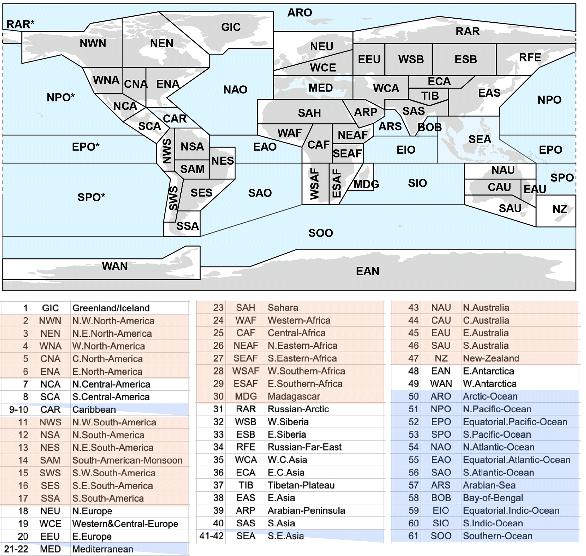
Figure B1. Map and lookup table for IPCC regional codes

Table B1. Regional Lookup Table of Disturbance Risk (This table currently displays a subset of regions as an example and will be comprehensive after public review)

Region	Indicator	Variable	Time	Value	Risk	Score
Eastern North America (ENA)	Temperature	Frost Days	Historical	116	High	0.5
		Days > 40℃	Historical	0.1	Low	0
		Days > 40℃	Change (Days)	0.6	Low	0
	Hydrological	CDD	Historical	15.5	Low	0
		CDD	Change (Days)	-0.3	Low	0
		5-Day Precipitation	Historical	89.4	Medium	0.25
		5-Day Precipitation	Change (%)	9	Low	0

Table B2. Global Benchmark Values for Extreme Weather Risks.

Time Frame	Variable	Median	75th%	90th%
Historical	Frost Days	89.8	94.1	97.5
	Days Max Temp > 40°C	9.9	15.1	21.9
	Consecutive Dry Days	63.7	71	76.2
	Maximum 5-day Precipitation (mm)	79.5	86	90.4
Projected Future	Frost Days	-	-	-
	Days Max Temp > 40°C	9.9	11.8	14.6
	Consecutive Dry Days	0.3	1.1	1.8
	Maximum 5-day Precipitation (%)	8.9	11.5	14.1

13.0

Appendix C: Buffer Pool Contributions

By default, Projects are subject to a flat 20% Buffer Pool contribution as outlined in Section 10.4.1 of the Improved Forest Management Protocol. Project Proponents may opt to calculate a project-specific Buffer Pool contribution based on the outputs of their Risk Assessment (Appendix A) for each Reporting Period.

The following steps are used to convert the outputs of the Risk Assessment into a Buffer Pool contribution:

Sum the total score for each risk category in Table A1.
Map the risk score for each risk category into a Buffer Pool contribution using Table C1.
Sum the Buffer Pool contribution for each risk category to obtain the total Buffer Pool contribution.

Table C1. Risk score to Buffer Pool contribution conversion for each risk category.

Risk Category	Cumulative Risk Score	Buffer Pool Contribution
Project Proponent Capacity Risk	0	2.0
	1	2.2
	2	2.7
	3	4.0
	4	6.0
	5	7.3
	6	7.8
	7	8.0
Financial Viability Risk	0	2.0
	1	2.2
	2	2.7
	3	4.0
	4	6.0
	5	7.3
	6	7.8
	7	8.0
Social Governance Risk	0	2.0
	1	2.2
	2	2.5
	3	3.1
	4	4.3
	5	5.7
	6	6.9
	7	7.5
	8	7.8
	9	8.0
Disturbance Risk	0	2.0
	1	2.1
	2	2.3
	3	2.5
	4	2.8
	5	3.4
	6	4.1
	7	5.0
	8	5.9
	9	6.6
	10	7.2
	11	7.5
	12	7.7
	13	7.9
	14	8.0

The Buffer Pool contribution for each risk category is determined using a sigmoid function described by Equation C1. The Buffer Pool contribution for each risk category ranges from 2% to 8%.

 $BP_{risk}=\frac{L}{1+e^{-k(x-x_0)}}+2$

(Equation C1)

Where:

$BP_{risk}$ is the Buffer Pool contribution for a given risk category.
$L=6$ is the range of Buffer Pool contributions within each risk category (2% to 8%).
$k = \frac{10}{cutoff -1}$ is the steepness parameter of the sigmoid curve and determines how quickly the function transitions between its minimum and maximum values.
$x_0 = \frac{cutoff}{2}$ is the midpoint of the sigmoid curve.
$x$ is the risk score for a given risk category.
$cutoff$ is the value at which the Project fails the Risk Assessment, noted in Appendix A.

The sigmoid function, Equation C1, applied to each risk category can also be visualized in Figure C1.

Figure C1. Buffer Pool contribution based on risk score for each risk category.

13.1

Project-Specific Buffer Pool Contribution Example

The Project has completed the Risk Assessment and obtained the following risk scores in a Reporting Period:

Project Proponent Capacity Risk = 2
Financial Viability Risk = 4
Social Governance Risk = 3
Disturbance Risk = 3

Mapping these risk scores to Table C1, the total Buffer Pool contribution for the Project is:

2.7% + 6.0% + 3.1% + 2.5% = 14.3%

14.0

Appendix D: Implementation of the Global Timber Model

This appendix provides detailed information on how Isometric implements the Global Timber Model (GTM) for leakage assessment in this Module, including technical requirements, scalar values, and forest type-regional classifications used in the modeling process.

14.1

Model Implementation Overview

Isometric implements the Global Timber Model (GTM) to quantify leakage deductions for each Reporting Period based on global runs of leakage rates for forest-type regions, annualized and weighted by the Project's basal area (see Section 7.2). Currently, Isometric uses a 2023 version of the GTM published by Dr. Adam Daigneault at the University of Maine and collaborators from The Nature Conservancy.

14.2

GTM Scalar Values and Parameters

Isometric currently applies the scalar values and parameters found below in Table D1 in its GTM implementation.

Table D1. Summary Table of Key Scalars in GTM for Protocol Leakage Assessment

Scalar	Value	Same as used in Daigneault et al 2024 (in review)	Explanation
Annual discount rate	5.00%	Yes	Commonly assumed to represent the average expected rate of return in the global forest sector
Global carbon project implementation rate	4.00%	No	A conservative accounting of forest area unavailable for commercial harvest due to carbon projects; see detailed explanation below
Elasticity of management intensity to timber price	Variable	Yes	Set for each region
Elasticity of timber demand to timber price	-1.0	Yes	Substitutions occur over decade-long timesteps in GTM, and in aggregate are more likely than single substitutions in single years. See Sohngen 2024 for additional explanation.
Elasticity of land area in forest to timber price	0.3	Yes	Based on Lubowski et al. 2006, Sohngen et al. 2019

14.2.1

Global Carbon Project Implementation Rate Detail

To date, the GTM uses a global implementation rate representing the proportion of all forest land globally available for harvest that is enrolled in forest carbon projects. Isometric determines harvest eligibility by accessibility, i.e., all accessible forests are eligible. However, Isometric has excluded forest area reported in the FAO Forest Resources Assessment as "protected".

As of the certification of this Module, the total global area of land enrolled in forest carbon projects is 77.599 Mha, based on an analysis of all forest-based carbon projects recorded by Renoster as of June 3, 2024. This represents approximately 8% of the total available forest area, which is 982.5 Mha as of the certification of this Module.

Research by Haya et al. (2023)⁴^,¹¹, Stapp et al. (2023)¹², and others suggests that the majority of forest carbon projects greatly overestimate emission reductions and that enrollment in carbon projects has historically been unlikely to result in near-term reductions in harvesting or deforestation. Thus, Isometric applies a conservative estimate that the actual amount of carbon project land on which all harvest is prevented is 50% of the calculated implementation rate of 8%. Thus, Isometric applies a global carbon project implementation rate of 4% (Table D1).

14.3

Forest Type-Region Classifications

Isometric will match the species present in the Project area to a GTM forest type and region (Tables D2, D3). The forest types are based on the 2010 United Nations Food and Agriculture Organization (UN FAO) Global Ecological Zones (GEZs), with enhanced resolution for United States forest types based on USFS FIA Regional Groupings. If species or genus are not explicitly listed in the GTM forest types, consult authoritative sources including local foresters and wood-database.com to determine similar commercial use and ecological characteristics for matching.

Table D2. Forest type and region classification table for the United States

Forest Type	Region	Forest Type Description	Region Description
Pine	Southeast	Pine species grown naturally or commercially, including loblolly pine (Pinus taeda), slash pine (P. elliottii), longleaf pine (P. palustris), and shortleaf pine (P. echinata)	Virginia, North Carolina, South Carolina, Georgia, Florida, Alabama, Mississippi, Louisiana
EHW		Eastern non-oak hardwood species grown naturally or commercially, including sweetgum (Liquidambar styraciflua), yellow-poplar (Liriodendron tulipifera), and red maple (Acer rubrum)
Oak		Oak species (Quercus spp.) including white oak (Q. alba), northern red oak (Q. rubra), southern red oak (Q. falcata), and post oak (Q. stellata)
Pine	South-Central	Pine species including shortleaf pine (Pinus echinata), loblolly pine (P. taeda), and pitch pine (P. rigida)	Kentucky, Tennessee, Arkansas, Oklahoma
EHW		Eastern non-oak hardwood species including tulip tree (Liriodendron tulipifera), sweetgum (Liquidambar styraciflua), and black walnut (Juglans nigra)
Oak		Oak species including white oak (Quercus alba), black oak (Q. velutina), and chestnut oak (Q. prinus)
SF	Northeast	Spruce-fir forest types including red spruce (Picea rubens), balsam fir (Abies balsamea), and eastern hemlock (Tsuga canadensis)	Maine, New Hampshire, Vermont, Massachusetts, Rhode Island, Connecticut, New York, Pennsylvania
Pine		Northern pine species including eastern white pine (Pinus strobus), red pine (P. resinosa), and jack pine (P. banksiana)
EHW		Eastern hardwood species including sugar maple (Acer saccharum), American beech (Fagus grandifolia), and yellow birch (Betula alleghaniensis)
Oak		Oak species including northern red oak (Quercus rubra), white oak (Q. alba), and chestnut oak (Q. prinus)
SF	North-Central	Spruce-fir complexes including white spruce (Picea glauca), balsam fir (Abies balsamea), and northern white-cedar (Thuja occidentalis)	Minnesota, Wisconsin, Michigan, Iowa, Missouri, Illinois, Indiana, Ohio
Pine		Northern pine species including red pine (Pinus resinosa), jack pine (P. banksiana), and eastern white pine (P. strobus)
EHW		Hardwood species including sugar maple (Acer saccharum), American basswood (Tilia americana), and northern red oak (Quercus rubra)
Oak		Oak species including bur oak (Quercus macrocarpa), white oak (Q. alba), and northern red oak (Q. rubra)
DF	West	Douglas-fir (Pseudotsuga menziesii) and associated coniferous species including western hemlock (Tsuga heterophylla) and grand fir (Abies grandis)	California, Oregon, Washington
Pine		Western pine species including ponderosa pine (Pinus ponderosa), sugar pine (P. lambertiana), and lodgepole pine (P. contorta)
HW		Western hardwood species including red alder (Alnus rubra), bigleaf maple (Acer macrophyllum), and Oregon white oak (Quercus garryana)
SW		Softwood species other than Douglas-fir and pine, including western redcedar (Thuja plicata), western hemlock (Tsuga heterophylla), and true fir species (Abies spp.)
HW	Southwest	Southwestern hardwood species including Fremont cottonwood (Populus fremontii), Arizona sycamore (Platanus wrightii), and Gambel oak (Quercus gambelii)	Texas, New Mexico, Arizona
DF	Southwest	Douglas-fir (Pseudotsuga menziesii) adapted to southwestern growing conditions	Texas, New Mexico, Arizona
Pine	Mountain	Mountain pine species including ponderosa pine (Pinus ponderosa), lodgepole pine (P. contorta), and limber pine (P. flexilis)	Montana, Wyoming, Colorado, Idaho, Nevada, Utah
HW	Mountain	Mountain hardwood species including quaking aspen (Populus tremuloides), Rocky Mountain maple (Acer glabrum), and paper birch (Betula papyrifera)	Montana, Wyoming, Colorado, Idaho, Nevada, Utah

Table D3. Forest type and region classification table for Countries and regions excluding the United States.

Forest Type	Region	Forest Type Description	Region Description
Plantation	China	Fast-growing plantation species including eucalyptus (Eucalyptus spp.), poplar (Populus spp.), and Chinese fir (Cunninghamia lanceolata) under intensive management	All administrative regions with forest plantation development
Natural	China	Natural forest ecosystems including mixed temperate forests, boreal forests, and subtropical forests with native species composition
S. Plt.	Brazil	Short-rotation plantation forestry focused on eucalyptus (Eucalyptus spp.) and pine (Pinus spp.) for industrial wood production	All states with plantation forestry operations
Trop. Evergreen		Tropical evergreen rainforest including Amazon rainforest with diverse hardwood species	Primarily Amazon Basin states
Trop. Mixed		Tropical mixed forests including Atlantic Forest remnants and Cerrado formations	Atlantic coast regions and central Cerrado
Atlantic/MW HW	Canada	Atlantic and Maritime hardwood forests including sugar maple (Acer saccharum), yellow birch (Betula alleghaniensis), and American beech (Fagus grandifolia)	Atlantic Maritime provinces
Atlantic/MW SW		Atlantic and Maritime softwood forests dominated by red spruce (Picea rubens), balsam fir (Abies balsamea), and eastern hemlock (Tsuga canadensis)
Atlantic/MW Mx		Atlantic and Maritime mixed forests combining hardwood and softwood species
Boreal/Hudson HW		Boreal hardwood forests including paper birch (Betula papyrifera), trembling aspen (Populus tremuloides), and balsam poplar (P. balsamifera)	Hudson Bay lowlands region
Boreal/Hudson SW		Boreal softwood forests including black spruce (Picea mariana), white spruce (P. glauca), and jack pine (Pinus banksiana)
Boreal/Hudson MX		Boreal mixed forests combining deciduous and coniferous species in the Hudson Bay region
Taiga HW		Northern taiga hardwood species including paper birch (Betula papyrifera) and trembling aspen (Populus tremuloides)	Northern territories and provinces
Taiga SW		Taiga softwood forests dominated by black spruce (Picea mariana) and tamarack (Larix laricina)
Taiga Mx		Taiga mixed forests combining hardwood and softwood species in extreme northern climates
Boreal West HW		Western boreal hardwood forests including trembling aspen (Populus tremuloides), balsam poplar (P. balsamifera), and paper birch (Betula papyrifera)	Western boreal regions
Boreal West SW		Western boreal softwood forests including white spruce (Picea glauca), black spruce (P. mariana), and lodgepole pine (Pinus contorta)
Boreal West MX		Western boreal mixed forests representing transitions between hardwood and softwood stands
Boreal Montane HW		Montane boreal hardwood forests including trembling aspen (Populus tremuloides) and paper birch (Betula papyrifera)	Rocky Mountain and cordilleran regions
Boreal Montane SW		Montane boreal softwood forests including subalpine fir (Abies lasiocarpa), Engelmann spruce (Picea engelmannii), and lodgepole pine (Pinus contorta)
Boreal Montane Mx		Mixed montane boreal forests combining elevation-adapted hardwood and softwood species
Pacific HW		Pacific coast hardwood forests including red alder (Alnus rubra) and bigleaf maple (Acer macrophyllum)	British Columbia coastal regions
Pacific SW		Pacific coast softwood forests dominated by western hemlock (Tsuga heterophylla), western redcedar (Thuja plicata), and Douglas-fir (Pseudotsuga menziesii)
Pacific Mx		Pacific coast mixed forests combining coastal hardwood and softwood species
Conifer	Russia	Russian coniferous forests including Siberian pine (Pinus sibirica), Siberian spruce (Picea obovata), and Siberian fir (Abies sibirica)	Siberian and Far East regions
Temp HW		Temperate hardwood forests including birch (Betula spp.), aspen (Populus spp.), and oak species (Quercus spp.)	European Russia and southern regions
Bor HW		Boreal hardwood forests dominated by birch (Betula spp.) and aspen (Populus spp.)	Northern boreal zone
HW		General hardwood forest classification for mixed deciduous species	Various regions with hardwood forest presence
Nord. Plt.	European Union	Nordic plantation forestry including Norway spruce (Picea abies), Scots pine (Pinus sylvestris), and managed species	Scandinavia and northern European countries
Ce.S. Plt.		Central European softwood plantations including Norway spruce (Picea abies) and silver fir (Abies alba)	Germany, Austria, Czech Republic, and surrounding regions
Ce.H.Plt.		Central European hardwood plantations including European beech (Fagus sylvatica) and oak species (Quercus spp.)	Germany, Austria, Czech Republic, and surrounding regions
So.S.Plt.		Southern European softwood plantations including maritime pine (Pinus pinaster) and stone pine (P. pinea)	Mediterranean countries
So.H.Plt.		Southern European hardwood plantations including cork oak (Quercus suber), holm oak (Q. ilex), and eucalyptus (Eucalyptus spp.)	Mediterranean countries
E. SW		Eastern European softwood forests including Norway spruce (Picea abies) and Scots pine (Pinus sylvestris)	Eastern European member states
E. HW		Eastern European hardwood forests including European beech (Fagus sylvatica), oak species (Quercus spp.), and hornbeam (Carpinus betulus)	Eastern European member states
Temp HW	Europe (Non-EU)	Temperate hardwood forests in non-EU European countries including beech (Fagus spp.) and oak (Quercus spp.)	Non-EU European countries including Switzerland, Norway, and Balkans
Temp SW		Temperate softwood forests including Norway spruce (Picea abies) and Scots pine (Pinus sylvestris)
Temperate Mixed		Mixed temperate forests combining hardwood and softwood species
LR PLT	South Asia	Large-rotation plantation forestry including teak (Tectona grandis) and sal (Shorea robusta)	India, Pakistan, Bangladesh, and surrounding countries
Tropical	South Asia	Tropical forests including monsoon forests, dry deciduous forests, and wet evergreen forests	India, Pakistan, Bangladesh, and surrounding countries
S PLT	Central America	Small-scale plantation forestry including coffee shade trees and mahogany (Swietenia spp.)	Mexico, Guatemala, Belize, Honduras, El Salvador, Nicaragua, Costa Rica, Panama
TMP EVER		Temperate evergreen forests including cloud forests and pine-oak forests
TMP MX		Temperate mixed forests combining coniferous and deciduous species
TMP DC		Temperate deciduous forests including oak forests and mixed deciduous formations
S PLT	Rest of South America	Short-rotation plantation forestry including eucalyptus (Eucalyptus spp.) and pine (Pinus spp.)	Countries other than Brazil
TR EVER		Tropical evergreen rainforests including Amazon basin forests
TR MIX		Tropical mixed forests including seasonal dry forests and forest-savanna mosaics
TEMP MX		Temperate mixed forests including Valdivian rainforest and Andean mixed forests
S PLT	Sub-Saharan Africa	Short-rotation plantation forestry including eucalyptus (Eucalyptus spp.) and wattle (Acacia spp.)	African countries south of the Sahara Desert
TR EV		Tropical evergreen forests including Congo Basin rainforests and East African montane forests
TR MIX		Tropical mixed forests including miombo woodlands and moist forests
Dipt	Southeast Asia	Dipterocarp forests dominated by Dipterocarpaceae family species characteristic of Southeast Asian rainforests	Indonesia, Malaysia, Thailand, Philippines, Vietnam, and surrounding countries
Trop. Dry		Tropical dry forests including monsoon forests and deciduous forests
Trop. Moist		Tropical moist forests including lowland rainforests and wet evergreen formations
S. Plt.		Short-rotation plantation forestry including oil palm (Elaeis guineensis), rubber (Hevea brasiliensis), and timber species
Temp	Oceania	Temperate forests including sclerophyll forests and wet temperate rainforests	Australia, New Zealand, and Pacific Islands
Trop. Dry		Tropical dry forests and woodlands adapted to seasonal rainfall
Trop. Moist		Tropical moist forests including wet tropical rainforests
S. Plt.		Short-rotation plantation forestry including eucalyptus (Eucalyptus spp.) and pine (Pinus spp.)
Temperate	Japan	Temperate forests including deciduous broad-leaved forests and mixed forests	All prefectures
S PLT	Japan	Short-rotation plantation forestry including Japanese cedar (Cryptomeria japonica) and other managed species	All prefectures
TR EVER	Africa and Middle East	Tropical evergreen forests in limited areas with suitable tropical climate	Limited tropical forest areas
TR MIX	Africa and Middle East	Tropical mixed forests and woodlands including dry forests and savanna-forest transitions	Various countries in Africa and Middle East

15.0

Acknowledgements

Isometric would like to thank Renoster, for their extensive feedback during this Module's development.

16.0

Definitions and Acronyms

Above Ground Biomass (AGB)The total mass of living woody biomass existing above the soil surface in a specified area.
ActivityThe steps of a Project Proponent’s Removal or Reduction process that result in carbon fluxes. The carbon flux associated with an activity is a component of the Project Proponent’s Protocol.
AdditionalityAn evaluation of the likelihood that an intervention—for example, a CDR Project—causes a climate benefit above and beyond what would have happened in a no-intervention Baseline scenario.
BaselineA set of data describing pre-intervention or control conditions to be used as a reference scenario for comparison.
Below Ground Biomass (BGB)The total mass of living woody biomass existing below the soil surface in a specified area.
BiodiversityThe diversity of life across taxonomic and spatial scales. Biodiversity can be measured within species (i.e. genetic diversity and variations in allele frequencies across populations), between species (i.e. the total number and abundance of species within and across defined regions), within ecosystems (i.e. the variation in functional diversity, such as guilds, life-history traits, and food-webs), and between ecosystems (variation in the services of abiotic and biotic communities across large, landscape-level scales) that support ecoregions and biomes.
Buffer PoolA common and recognized insurance mechanism among Registries allowing Certificates to be set aside (in this case by Isometric) to compensate for Reversals which may occur in the future.
Carbon Dioxide Equivalent Emissions (CO₂e)The amount of CO₂ emissions that would cause the same integrated radiative forcing or temperature change, over a given time horizon, as an emitted amount of GHG or a mixture of GHGs. One common metric of CO₂e is the 100-year Global Warming Potential.
Carbon Dioxide Removal (CDR)Activities that remove carbon dioxide (CO₂) from the atmosphere and store it in products or geological, terrestrial, and oceanic Reservoirs. CDR includes the enhancement of biological or geochemical sinks and direct air capture (DAC) and storage, but excludes natural CO₂ uptake not directly caused by human intervention.
Carbon FinanceResources provided to projects that are generating, or are expected to generate, greenhouse gas (GHG) Emission Reductions or Removals.
Certification (of a Protocol)The Isometric process which involves expert review and Public Consultation in order to arrive at an approved version of a Protocol, against which Projects will be Validated and Removals or Reductions will be Verified.
ConservativePurposefully erring on the side of caution under conditions of Uncertainty by choosing input parameter values that will result in a lower net CO₂ Removal or GHG Reduction than if using the median input values. This is done to increase the likelihood that a given Removal or Reduction calculation is an underestimation rather than an overestimation.
CounterfactualAn assessment of what would have happened in the absence of a particular intervention – i.e., assuming the Baseline scenario.
Cradle-to-GraveConsidering impacts at each stage of a product's life cycle, from the time natural resources are extracted from the ground and processed through each subsequent stage of manufacturing, transportation, product use, and ultimately, disposal.
CreditA publicly visible uniquely identifiable Credit Certificate Issued by a Registry that gives the owner of the Credit the right to account for one net metric tonne of Verified CO₂e Removal or Reduction. In the case of this Standard, the net tonne of CO₂e Removal or Reduction comes from a Project Validated against a Certified Protocol.
Crediting PeriodThe period of time over which a Project Design Document is valid, and over which Removals, Reductions or Environmental Attributes may be Verified, resulting in Issued Certificates.
DurabilityThe amount of time carbon removed from the atmosphere by an intervention – for example, a CDR project – is expected to reside in a given Reservoir, taking into account both physical risks and socioeconomic constructs (such as contracts) to protect the Reservoir in question.
Dynamic BaseliningA method for establishing and regularly updating the reference carbon stock levels in a reforestation project area, based on ongoing analysis of comparable non-project plots, to account for natural fluctuations and improve the accuracy of carbon Certificate calculations over the project lifetime.
Ecological IntegrityThe ability of an ecosystem to support and maintain ecological processes and a diverse community of organisms. It is measured as the degree to which a diverse community of native organisms is maintained, and is used as a proxy for ecological resilience, intended as the capacity of an ecosystem to adapt in the face of stressors, while maintaining the functions of interest.
Ecosystem FunctionThe natural processes and interactions that occur within an ecosystem, including the flow of energy and materials through biotic and abiotic components, encompassing activities like nutrient cycling, primary production, and habitat provision, which collectively maintain the balance and stability of the ecosystem.
Emission ReductionsLowering future GHG releases from a specific entity.
EmissionsThe term used to describe greenhouse gas emissions to the atmosphere as a result of Project activities.
Financial AdditionalityAn evaluation of the likelihood that an intervention that causes a climate benefit above and beyond what would have happened in a no-intervention Baseline scenario was the result of revenues from carbon finance.
Greenhouse Gas (GHG)Those gaseous constituents of the atmosphere, both natural and anthropogenic (human-caused), that absorb and emit radiation at specific wavelengths within the spectrum of terrestrial radiation emitted by the Earth’s surface, by the atmosphere itself, and by clouds. This property causes the greenhouse effect, whereby heat is trapped in Earth’s atmosphere (CDR Primer, 2022).
International Standards Organization (ISO)A worldwide federation (NGO) of national standards bodies from more than 160 countries, one from each member country.
Invasive SpeciesA species whose introduction, spread, and/or growth threatens biological diversity.
Issuance (of a Certificate)Certificates are issued to the Certificate Account of a Project Proponent with whom Isometric has a Validated Protocol after an Order for Verification and Certificate Issuance services from a Buyer and once a Verified Removal or Reduction has taken place.
LeakageThe increase in GHG emissions outside the geographic or temporal boundary of a project that results from that project's activities.
Light Detection and Ranging (LiDAR)LiDAR is a remote sensing technology that uses laser pulses to create highly accurate three-dimensional maps of forest structure, enabling measurements of tree height, canopy density, and biomass.
Lossesfor open systems, biogeochemical and/or physical interactions which occur during the removal process that decrease the CO₂ removal .
ModelA calculation, series of calculations or simulations that use input variables in order to generate values for variables of interest that are not directly measured.
ModuleIndependent components of Isometric Certified Protocols which are transferable between and applicable to different Protocols.
ProjectAn activity or process or group of activities or processes that alter the condition of a Baseline and leads to Removals or Reductions.
Project Design DocumentThe document, written by a Project Proponent, which records key characteristics of a Project and which forms the basis for Project Validation and evaluation in accordance with the relevant Certified Protocol. (Also known as “PDD”).
Project Design Document (PDD)The document that clearly outlines how a Project will generate rigorously quantifiable Additional high-quality Removals or Reductions.
Project ProponentThe organization that develops and/or has overall legal ownership or control of a Removal or Reduction Project.
Project boundaryThe defined temporal and geographical boundary of a Project.
ProtocolA document that describes how to quantitatively assess the net amount of CO₂ removed by a process. To Isometric, a Protocol is specific to a Project Proponent's process and comprised of Modules representing the Carbon Fluxes involved in the CDR process. A Protocol measures the full carbon impact of a process against the Baseline of it not occurring.
ProxyA measurement which correlates with but is not a direct measurement of the variable of interest.
RPReporting Period
RegistryA database that holds information on Verified Removals and Reductions, and reviewed EACs, based on Protocols. Registries Issue Certificates, and track their ownership and Retirement.
Remote SensingThe use of satellite, aircraft and terrestrial deployed sensors to detect and measure characteristics of the Earth's surface, as well as the spectral, spatial and temporal analysis of this data to estimate biomass and biomass change.
RemovalThe term used to represent the CO₂ taken out of the atmosphere as a result of a CDR process.
ReversalThe escape of CO₂ to the atmosphere after it has been stored, and after a Certificate has been Issued. A Reversal is classified as avoidable if a Project Proponent has influence or control over it and it likely could have been averted through application of reasonable risk mitigation measures. Any other Reversals will be classified as unavoidable.
StakeholderAny person or entity who can potentially affect or be affected by Isometric or an individual Project activity.
StorageDescribes the addition of carbon dioxide removed from the atmosphere to a reservoir, which serves as its ultimate destination. This is also referred to as “sequestration”.
Synthetic Aperture Radar (SAR)A remote sensing technology which uses radio waves to create images of the earth’s surface.
USDAUnited States Department of Agriculture
UncertaintyA lack of knowledge of the exact greenhouse gas impact (removal, reduction, or avoidance) associated with a particular process or Environmental Attribute. Uncertainty may be quantified using probability distributions, confidence intervals, or variance estimates.
ValidationA systematic and independent process for evaluating the reasonableness of the assumptions, limitations and methods that support a Project and assessing whether the Project conforms to the criteria set forth in the Isometric Standard and the Protocol by which the Project is governed. Validation must be completed by an Isometric approved third-party (VVB).
Validation and Verification Bodies (VVBs)Third-party auditing organizations that are experts in their sector and used to determine if a project conforms to the rules, regulations, and standards set out by a governing body. A VVB must be approved by Isometric prior to conducting validation and verification.
VerificationA process for evaluating and confirming the net Removals and Reductions for a Project, using data and information collected from the Project and assessing conformity with the criteria set forth in the Isometric Standard and the Protocol by which it is governed. Verification must be completed by an Isometric approved third-party (VVB).

17.0

References

Butler, B., Hewes, J. H., Dickinson, B. J., Andrejczyk, K., Butler, S. M., & Markowski-Lindsay, M. (2016). USDA Forest Service National Woodland Owner Survey: national, regional, and state statistics for family forest and woodland ownerships with 10+ acres, 2011-2013. Res. Bull. NRS-99. Newtown Square, PA: US Department of Agriculture, Forest Service, Northern Research Station. 39 p., 99, 1-39. https://doi.org/10.2737/NRS-RB-99 ↩
Silver, E. J., Leahy, J. E., Weiskittel, A. R., Noblet, C. L., & Kittredge, D. B. (2015). An evidence-based review of timber harvesting behavior among private woodland owners. Journal of Forestry, 113(5), 490-499. https://doi.org/10.5849/jof.14-089 ↩
Badgley, G., Freeman, J., Hamman, J. J., Haya, B., Trugman, A. T., Anderegg, W. R., & Cullenward, D. (2022). Systematic over‐crediting in California's forest carbon offsets program. Global Change Biology, 28(4), 1433-1445. https://doi.org/10.1111/gcb.15943 ↩
Haya, B. K., Evans, S., Brown, L., Bukoski, J., Butsic, V., Cabiyo, B., ... & Sanchez, D. L. (2023). Comprehensive review of carbon quantification by improved forest management offset protocols. Frontiers in Forests and Global Change, 6, 958879. https://doi.org/10.3389/ffgc.2023.958879 ↩ ↩²
Haya, B. (2019). The California Air Resources Board's U.S. Forest Offset Protocol Underestimates Leakage. University of California, Berkeley. Available online at: https://gspp.berkeley.edu/assets/uploads/research/pdf/Policy_Brief-US_Forest_Projects-Leakage-Haya_4.pdf (accessed September 15, 2025) ↩
Sohngen, B., Mendelsohn, R., & Sedjo, R. (1999). Forest management, conservation, and global timber markets. American Journal of Agricultural Economics, 81(1), 1-13. https://doi.org/10.2307/1244446 ↩
Gao, S., Zhong, R., Yan, K., Ma, X., Chen, X., Pu, J., ... & Myneni, R. B. (2023). Evaluating the saturation effect of vegetation indices in forests using 3D radiative transfer simulations and satellite observations. Remote Sensing of Environment, 295, 113665. https://doi.org/10.1016/j.rse.2023.113665 ↩
An initial evaluation of carbon proxies for dynamic reforestation baselines. Pachama. Retrieved October 16, 2024, from https://pachama.com/blog/dynamic-reforestation-baselines/ ↩
Wilkinson, M. D., Dumontier, M., Aalbersberg, I. J., Appleton, G., Axton, M., Baak, A., ... & Mons, B. (2016). The FAIR Guiding Principles for scientific data management and stewardship. Scientific Data, 3(1), 1-9. https://doi.org/10.1038/sdata.2016.18 ↩
IPCC, 2023: Climate Change 2023: Synthesis Report. Contribution of Working Groups I, II and III to the Sixth Assessment Report of the Intergovernmental Panel on Climate Change [Core Writing Team, H. Lee and J. Romero (eds.)]. IPCC, Geneva, Switzerland, pp. 35-115. https://doi.org/10.59327/IPCC/AR6-9789291691647 ↩
Haya, B. K., Alford-Jones, K., Anderegg, W. R., Beymer-Farris, B., Blanchard, L., & Bomfim, B. (2023). Quality assessment of REDD+ carbon credit projects. https://gspp.berkeley.edu/assets/uploads/page/Quality-Assessment-of-REDD+-Carbon-Crediting.pdf ↩
Stapp, J., Nolte, C., Potts, M., Baumann, M., Haya, B. K., & Butsic, V. (2023). Little evidence of management change in California’s forest offset program. Communications Earth & Environment, 4(1), 331. https://doi.org/10.1038/s43247-023-00984-2 ↩

Contributors

Christopher Kilner, Ph.D.

Ryan Huang, Ph.D.

Jeannie Wilkening, Ph.D.

Emma Marsland

Michael Shell

Isometric

Contents

Introduction

Sources and Reference Standards & Methodologies

Future Versions

Applicability

Viability of the Project and Determination of the Project Area

Land Enrollment and Parcel Classes

Integrity of Enrolled Land

Parcel Classes

Ecological Feasibility of Harvest

Soil Drainage Limitations

Seasonal Operability Exception

Proximity to Water Bodies

Geographical Constraints

Proximity to Dwellings and Other Structures

Merchantable Stocking

Quantification of Initial Carbon Stock

Other Requirements

Project Timelines

Crediting Period

Reporting Period

Environmental and Social Safeguarding

Safeguarding of Biodiversity

Forest Management Activities

Stand Improvement Activities

Harvesting Plan

Safeguarding of Community Livelihoods

Stakeholder Engagement

Community Impacts and Well-being

Relation to Isometric Standard

Additionality

Ecological Feasibility of Harvest

System Boundary, Project Baseline and Leakage

Leakage

Scientific Justification for a Unified Conservative Modeling Framework

Global Timber Model Implementation

Regional Leakage Rate Calculation

Project Leakage Calculation

Net CDR Quantification

Calculation of CO2eStored, RP

Calculation of MAGB

Calculation of MAGB through Growth-Disturbance Models

Growth Model

Disturbance Model

Carbon Stock Acquisition

Calculation of Baseline, CO2eCounterfactual, RP

Determination of Zone of Eligibility for Control Plots

Generation of Forest Carbon Map

Matching of Project and Control Pixels

Evaluation of Dynamic Baseline Deduction

Evaluation of Dynamic Baseline Uncertainty

Calculation of CO2eEmissions, RP

Model Validation Requirements

Storage and Durability of CO2e Removals

Durability

Durability Standardization

Appendix A: Risk Assessment

Appendix B: Calculating Extreme Weather Risk Scores

Appendix C: Buffer Pool Contributions

Project-Specific Buffer Pool Contribution Example

Appendix D: Implementation of the Global Timber Model

Model Implementation Overview

GTM Scalar Values and Parameters

Global Carbon Project Implementation Rate Detail

Forest Type-Region Classifications

Acknowledgements

Definitions and Acronyms

References

Footnotes

Contributors

Calculation of CO₂e_{Stored, RP}

Calculation of M_AGB

Calculation of M_AGB through Growth-Disturbance Models

Calculation of Baseline, CO₂e_{Counterfactual, RP}

Calculation of CO₂e_{Emissions, RP}

Storage and Durability of CO₂e Removals