Contents
1.0
Introduction
This module outlines the requirements for quantifying loss of alkalinity and/or CO2 to the atmosphere due to natural processes occurring in rivers and oceans, for Carbon Dioxide Removal (CDR) pathways that enhance alkalinity in the natural Earth system. Alkalinity represents the capacity of water to neutralize acids, dominated by bicarbonate (HCO3-) and carbonate (CO32-) ions in natural waters. The efficacy of carbon dioxide removal (CDR) methods that rely on alkalinity enhancement in the Earth system is dependent on the transport of that alkalinity through river networks to the ocean. As alkalinity-rich water traverses from rivers to the ocean, alkalinity can be lost from the system via the removal of HCO3- and CO32- ions from solution through various processes, predominantly:
- Carbonate mineral precipitation (inorganic or biologically mediated)
- Inorganic: in rivers and estuaries, mixing of fresh and saline water can change carbonate saturation state, leading to carbonate mineral precipitation1,2,3,4. This process consumes HCO3- and CO32- ions, reducing alkalinity.
- Biologically mediated: calcifying organisms (biota that make their shells from carbonate minerals) in estuaries and oceans consume alkalinity through CaCO3 formation.5
- CO2 outgassing
- When CO2 degasses, for example from turbulent water flows or photosynthesis-driven low pH conditions, the equilibrium of the carbonate system shifts, and HCO3- and CO32- can convert to CO2. This dissolved CO2 can be released to the atmosphere as a gas, reducing alkalinity in waters.6
- Changes in natural alkalinity fluxes
This Module standardizes the quantification of these loss processes across CDR pathways that enhance alkalinity in aquatic and hydrologic systems (groundwater, rivers, and the ocean), ensuring a consistently rigorous standard in how river and ocean losses are quantified and reported. This Module will be adapted as science evolves and will be reviewed regularly following the cadence set out in the Isometric Standard.
Throughout this Module, use of the word "must" indicates a requirement, whereas "should" indicates a recommendation.
2.0
Applicability
This Module applies to Projects that enhance alkalinity in the Earth system via one of the following Protocols and/or Modules:
- Enhanced Weathering in Agriculture Protocol
- Open System Ex-situ Mineralization Protocol
- River Alkalinity Enhancement Protocol
- Wastewater Alkalinity Enhancement Protocol
- Electrolytic Seawater Mineralization Protocol
- Ocean Alkalinity Enhancement from Coastal Outfalls Protocol
- Direct Ocean Capture and Storage Protocol
- Enhanced Weathering in Closed Engineered Systems Module
All GHG accounting and quantification of net carbon removal that occurs upstream and downstream of river and ocean losses must be carried out according to one of the Protocols and/or Modules listed above.
2.1
Eligibility Criteria for River Transport
This Module employs simplified assumptions for river transport and biogeochemistry to quantify losses in river transport. To ensure responsible application of this Module, the river must meet the following criteria unless otherwise specified in a Protocol:
- The transit time of the river reach must be under 45 days. The river transit time for losses is determined based on the shorter of the following distances:
- From where weathering products enter the river to the river mouth.
- From where removal quantification ends in the respective Protocol to the river mouth.
- For example, in WAE (Wastewater Alkalinity Enhancement) or Enhanced Weathering in Closed Engineered System Projects, this is from the discharge point to the river mouth, as removal quantification is calculated within the closed system prior to discharge.
- RAE (River Alkalinity Enhancement) Projects are required to directly measure river conditions downstream of initial mixing, so river losses and river transit time for losses apply from the last monitoring station for quantification to the river mouth.
- For Enhanced Weathering in Agriculture Projects, this would be the distance from the entry point of dissolved weathering products into the river through subsurface baseflow to the river mouth.
- The mean hydraulic residence time of all surface-water storage features (natural lakes and reservoirs combined) within the river reach must not exceed 3 days. Note that this applies to the river reach from the point of discharge into the river to the river mouth. Run-of-river structures without appreciable impoundment volume are permitted.
- The river must not discharge into salt marsh or mangrove dominated estuaries.
- Desert basins, closed lake systems, and ephemeral rivers that sink into karst or alluvial fans before reaching the coast are ineligible.
- Dosing at locations with downstream wastewater treatment facilities discharging directly into rivers may be eligible, subject to Isometric and VVB approval.
River eligibility must be demonstrated based on evidence such as:
- hydrologic gauge records or regional discharge models
- publicly available surface-water storage volume datasets
- established hydraulic routing or residence-time calculations
- remote sensing and coastal habitat maps to classify tidal wetlands and mangroves
- direct tracer studies are not required
If a Protocol has its own river eligibility criteria, the Protocol overrides this Module's eligibility criteria.
3.0
Relevant Loss Processes
The number and type of loss processes that must be quantified for a Project will differ depending on the CDR pathway and deployment location. Project Proponents must identify the relevant scenario from the flow chart in Figure 1, and see the corresponding Module section for the full list of loss processes that must be considered for their Project.
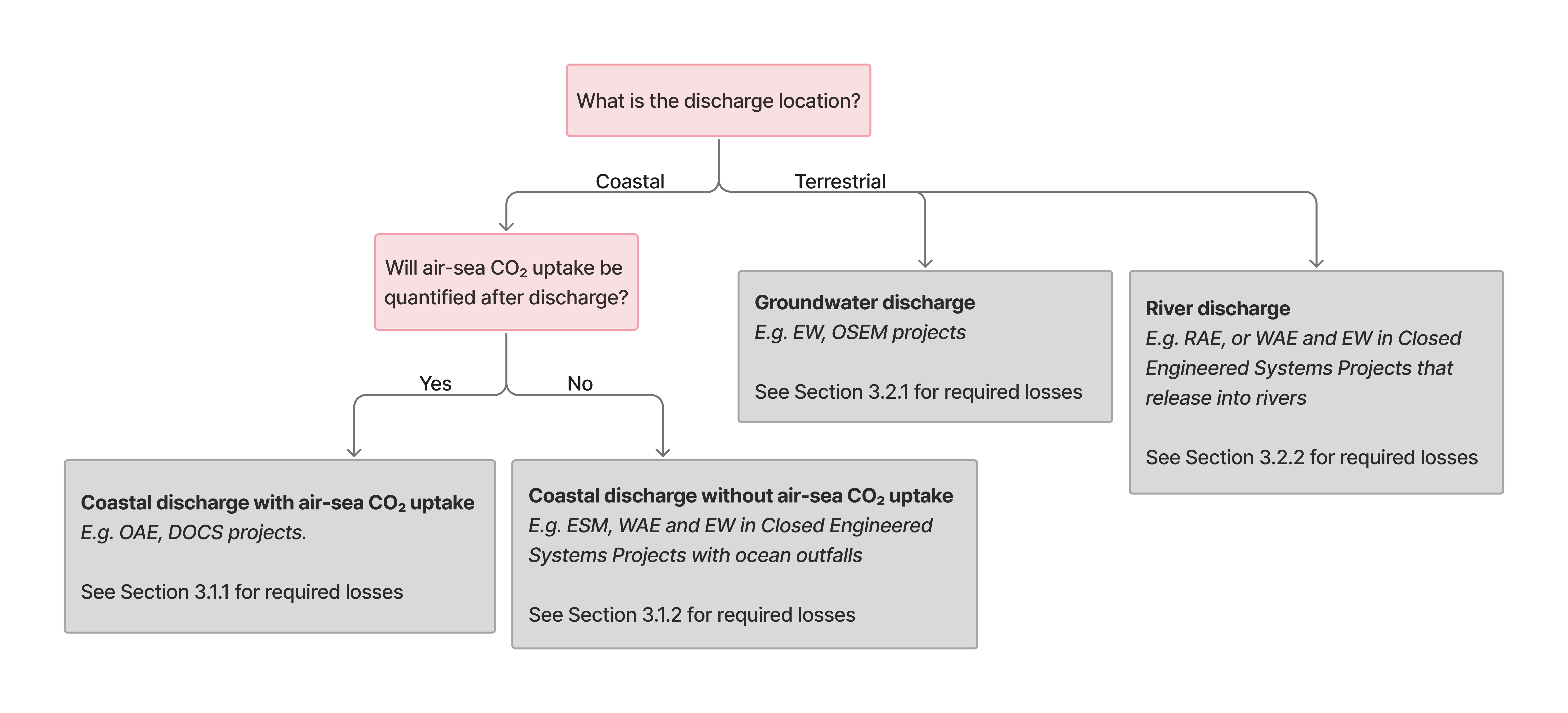
Figure 1 Flow chart for a Project to decide which list of losses are needed to be considered.
3.1
Coastal Discharge
The treatment of losses from Projects with coastal discharge will differ based on whether the effluent has equilibrated with the atmosphere or not prior to release into the ocean. This distinction determines which loss processes are applicable, and how the losses are applied during quantification of gross CDR.
3.1.1
Point-Source Coastal Discharge With Subsequent Air-Sea CO₂ Uptake
In Projects where the effluent is not equilibrated with the atmosphere prior to discharge, CO2 removal occurs after discharge in the ocean through air-sea gas exchange. This scenario applies to pathways such as Ocean Alkalinity Enhancement (OAE) and Direct Ocean Capture and Storage (DOCS). For these Projects, losses of alkalinity and/or DIC upon discharge will impact the air-sea CO2 drawdown potential, and must be quantified or demonstrated to be negligible prior to using the Air-Sea CO2 Uptake Module.
These Projects must include the following loss processes:
Ocean Losses
- Inorganic carbonate precipitation (Section 4.2.2)
- Natural alkalinity flux reduction (Section 4.2.3)
- Changes to biotic calcification (Section 4.2.4)
3.1.2
Point-Source Coastal Discharge Without Subsequent Air-Sea CO₂ Uptake
In Projects where the effluent is equilibrated with the atmosphere prior to discharge, CO2 is removed and quantified upstream of discharge. This scenario is relevant for pathways such as Electrolytic Seawater Mineralization (ESM), Enhanced Weathering in Closed Engineered Systems with ocean outfalls, and Wastewater Alkalinity Enhancement (WAE) with ocean outfalls. Subsequent losses upon entering the ocean must be quantified and deducted from gross carbon removal or robustly justified as negligible.
These Projects must include the following loss processes:
Ocean Losses
- Re-equilibration of the carbonate system upon entering the ocean (Section 4.2.1)
- Inorganic carbonate precipitation (Section 4.2.2)
- Natural alkalinity flux reduction (Section 4.2.3)
- Changes to biotic calcification (Section 4.2.4)
3.2
Terrestrial Discharge
Projects with terrestrial discharge include pathways such as Enhanced Weathering in Agriculture (EW), Open-System Ex-situ Mineralization (OSEM), and River Alkalinity Enhancement (RAE) or other Projects (such as Enhanced Weathering in Closed Engineered Systems and Wastewater Alkalinity Enhancement) that discharge directly into rivers. These pathways include removing and storing CO2 as Dissolved Inorganic Carbon (DIC) in porewater and/or receiving ground and surface waters which are eventually transported to the ocean for long term storage. Losses of CO2 may occur along the entire transport pathway from groundwater to rivers to the ocean. Accordingly, potential losses must be evaluated at each stage: within the soil profile to the water table, during groundwater transport, during riverine transport, and upon entering the ocean.
3.2.1
Diffuse Runoff
CO2 removed from pathways such as Enhanced Weathering in Agriculture (EW) or Open-System Ex-situ Mineralization (OSEM) is transported to rivers through runoff such as soil flow, surface runoff, lateral flow, and groundwater baseflow. This can collectively be represented as a diffuse discharge into rivers. This Module focuses on losses that occur in rivers and oceans only. Please see the relevant Protocols for details on quantifying losses in soils and groundwater (Enhanced Weathering in Agriculture Protocol).
These Projects must include the following loss processes:
River Losses
- Transport river losses
- Re-equilibration of the carbonate system (Section 4.1.1)
- This may be omitted if pH > 6 is maintained from the point of discharge into the river to the ocean.
- Inorganic carbonate precipitation (Section 4.1.2)
- Re-equilibration of the carbonate system (Section 4.1.1)
Ocean Losses
- Re-equilibration of the carbonate system upon entering the ocean (Section 4.2.1)
3.2.2
Point-Source River Discharge
Pathways with direct river discharge may include River Alkalinity Enhancement (RAE), Wastewater Alkalinity Enhancement (WAE) Projects and Enhanced Weathering in Closed Engineered Systems Projects.
These Projects must include the following losses:
River Losses
- Re-equilibration of the carbonate system (Section 4.1.1)
- This may be omitted if pH > 6 is maintained from the point of discharge to the river to the ocean.
- Inorganic carbonate precipitation (Section 4.1.2)
- Natural alkalinity flux reduction (Section 4.1.3)
- Additional (bio)geochemical sinks of alkalinity (Section 4.1.4)
Ocean Losses
- Re-equilibration of the carbonate system upon entering the ocean (Section 4.2.1)
4.0
Quantification of Losses
For each of the relevant loss processes identified from Section 3, Project Proponents must:
- Describe the risk of that loss process in the PDD (Project Design Document), and
- Provide one of the following:
- A justification of why the loss is negligible.
- This must include a description of the conditions which lead to a non-negligible loss, a description of how these conditions are avoided in the Project (e.g. staying below certain thresholds) and a plan for corresponding monitoring to demonstrate adherence to those guardrails.
- A strategy for quantifying a corresponding retention factor. Acceptable strategies for quantifying the impact of these loss processes include:
- Estimating a conservative upper limit of loss based on scientific literature, first principles calculations, and/or experimentation;
- Application of standardized default loss factor (conservatively from peer-reviewed literature) upon cross-checking eligible criteria through pre-screen;
- Process-based modeling studies;
- Direct measurements;
- Alternative approaches that are sufficiently justified.
- A justification of why the loss is negligible.
Data, measurements and evidence used in the quantification of loss factors must be publicly disclosed on the registry upon credit issuance. Specific requirements, as well as examples of acceptable justifications for when a certain process can be considered negligible, are provided for each of the loss processes below.
Sections 4.1 and 4.2 below outline the specific requirements and recommendations for each of the different loss processes in rivers and oceans. Much of the existing research in these losses have been motivated by research in Enhanced Weathering, River Liming, and Ocean Alkalinity Enhancement, which may not exactly simulate the carbonate chemistry state of the effluent from the different project types that this Module is applicable to. It is recommended that Project Proponents conduct additional site-specific studies to optimize loss estimates and research on the relevant carbonate chemistry parameters for their particular process conditions.
For Projects where carbon removal occurs before transport to the ocean, losses are defined as the fraction of carbon removal delivered to river systems that does not ultimately yield durable storage as DIC in the ocean. Non-negligible river and ocean losses must be quantified as a total retention factor that is applied to the gross CO2 removed.
The total retention factor is the product of the retention factors associated with each loss process:
(Equation 1)
Where:
- is the total retention factor for all relevant river and ocean loss processes. This factor is dimensionless with values between 0 and 1, and is applied to the gross CO2 removed.
- is the overall river retention factor, representing the fraction of CO2 retained after considering all relevant loss processes that occur in the river. This factor is dimensionless with values between 0 and 1.
- is the overall ocean retention factor, representing the fraction of CO2 retained after considering all relevant loss processes in the ocean. This factor is dimensionless with values between 0 and 1.
- A retention of 1 means 100% of the CO2 is retained (i.e. no losses), and a retention of 0 means none of the CO2 is retained for durable storage (i.e. all lost).
If the Project does not transit through any rivers, then the term is ignored and Equation 1 is just .
4.1
Riverine Losses
This section includes an overview of riverine loss processes and how to quantify them.
Quantification Requirements
Any non-negligible losses must be estimated and aggregated into a total riverine retention factor:
(Equation 2)
Where:
- represents the total fraction of CO2 retained upon reaching the river mouth before entering the ocean, dimensionless value between 0 and 1.
- is the fraction of CO2 that is retained after a given loss process, , dimensionless value between 0 and 1
- is the total number of loss processes.
Note that for RAE Projects, represents the losses from the last carbonate chemistry monitoring station to the river mouth. For all other Projects, represents the losses occurring upon entering the river and during transport to the river mouth.
This section covers the following riverine loss processes:
- Re-equilibration of the carbonate system
- Inorganic carbonate precipitation
- Natural alkalinity flux reduction
- Additional (bio)geochemical sinks of alkalinity
Note that not every process above is applicable to every Project. See Section 3 to determine the list of relevant processes for a specific Project.
Background
In rivers, total alkalinity (TA), which represents the acid-neutralizing capacity of the water, is dominated by bicarbonate and carbonate ions: TA HCO3- + 2CO32-. The addition of alkalinity from CDR Projects with terrestrial discharge shifts these equilibria, consuming protons (H+) and increasing the pH. This, in turn, shifts the speciation of DIC away from dissolved CO2 and towards bicarbonate HCO3- and carbonate CO32-, increasing the water's capacity to hold inorganic carbon. This increased "buffer capacity" is the central mechanism of alkalinity-based CDR.
Natural river systems are rarely in equilibrium with the atmosphere. Due to the influx of CO2-rich groundwater and the respiration of organic matter within the river channel and its floodplain, many of the world's rivers are naturally supersaturated with respect to atmospheric CO2 8,9. This means the partial pressure of CO2 (pCO2) in many rivers is higher than that of the atmosphere, making them natural sources of CO2 outgassing to the atmosphere10,11. Equilibrium assumptions should be applied conservatively when used to simplify the dynamics of gas exchange and mineral precipitation.
4.1.1
Re-Equilibration of the Carbonate System
Concept
Equilibrium speciation of DIC is primarily dependent on pH, and to a lesser extent temperature, salinity and pressure as shown in Equation 3.
(Equation 3)
The release of CO2 due to re-equilibration of DIC may occur due to mixing of fluids with different pH. This may occur upon initial dosing of alkalinity into a river, when groundwater enters a river, and at river confluences. The extent and rate of re-equilibration are highly site and project specific, depending on local water chemistry, hydrodynamic conditions, and effluent characteristics. If river gas transfer velocity is high, re-equilibration can be rapid. Conversely, in deep, slow-flowing, large rivers, the gas transfer velocity is much lower, and the water may travel for hundreds of kilometers without fully equilibrating with the atmosphere. Hydrology and pH are therefore both key variables controlling the potential for degassing losses.
Quantification
Quantification of riverine outgassing from re-equilibration is required when either the effluent pH or the pH of the mixed effluent and ambient water is less than 6 at any point in the river reach. This threshold is necessary because:
- For freshwater with pH ≥ 6, the carbon-capture retention factor based on enhanced alkalinity, defined as , is approximately equivalent to or higher than that of the ocean (Figure 2 adapted from Bertagni and Porporato (2022)12). In these cases, only losses of DIC due to inorganic carbonate precipitation will reduce carbon storage below the final ocean retention factor.
- However, for freshwater pH < 6, is less than the final ocean values (Figure 2). Outgassing during freshwater transport must be quantified in this scenario as it would not be captured by using the final ocean efficiencies alone.
Therefore, the pH < 6 threshold serves as a safeguard against over-crediting carbon removal.
When quantification is required (pH < 6), there are two contexts in which outgassing may occur:
- Initial mixing zone outgassing: Upon initial mixing of effluent with the receiving water body, rapid changes in water chemistry can drive CO2 outgassing. The recommended quantification approach is to use a two-endmember mixing model to estimate the DIC of the effluent and ambient water mixture. The difference between the measured DIC of the effluent and the calculated DIC of the mixture represents the the loss from CO2 outgassing, with additional loss occurring from carbonate precipitation. Isometric provides a default river loss model to quantify this, see Section 4.1.5.
- Outgassing during transport: Equilibrium models provide a conservative and generally acceptable framework for representing riverine CO₂ outgassing becasue they treat rivers as a series of batch reactors during downstream transport (see Section 4.1.6 for requirements for river transport models). However, in some river systems—particularly those with long residence times, shallow depths, or turbulent flow conditions, outgassing can occur as water travels toward the ocean. This is particularly relevant where the gas transfer velocity is high relative to travel time because these are conditions under which equilibrium assumptions may oversimplify CO2 losses. In such cases, inclusion of kinetic processes, such as gas transfer velocity, flow regime, and transport time between discharge and ocean delivery, can provide a more accurate assessment of CO2 evasion and alkalinity loss6.
Alternative quantification approaches may be used if they can be demonstrated to accurately capture the carbon losses under site-specific conditions.
Figure 2. Alkalinization Carbon-capture Efficiency (ACE), defined as , as a function of pH for natural waters. Figure is adapted from Bertagni and Porporato (2022)12 Figure 1. For seawater of 15 degrees and an average ocean pH of 8.1, is approximately 0.84, which is equal to the freshwater ACE at pH 6.
4.1.2
Inorganic Carbonate Precipitation
Concept
Secondary precipitation of carbonate minerals is a primary pathway for carbon loss. Typically secondary precipitation of calcium/magnesium carbonate, such as calcite (CaCO3), magnesite (MgCO3), and dolomite (CaMg(CO3)2) could cause CO2 outgassing by the following reaction as shown in Equation 4:
(Equation 4)
Calcium carbonate precipitation may result in a reduction in carbon loss up to 50% for non-carbonate feedstocks or up to 100% for carbonate feedstocks. This is because for every mole of calcite precipitated, two moles of alkalinity are consumed, and one mole of CO2 is released. The thermodynamic potential for this reaction to occur is described by the calcite saturation index (SIc) as shown in Equation 5 and Equation 6:
(Equation 5)
With:
(Equation 6)
Where:
- is the measured solution activities of those ions
- is the ion activity at saturation
When SIc > 0, the effluent is supersaturated and precipitation is thermodynamically favorable. However, a crucial distinction must be made between thermodynamic favorability and kinetic reality. The precipitation of calcite from solution is often kinetically inhibited, meaning it does not occur instantaneously even in supersaturated waters. Many natural river systems maintain a state of supersaturation SIc > 113,14,15 without significant precipitation occurring. Some studies suggest that extensive, rapid precipitation may only be triggered at a much higher kinetic threshold, such as when the saturation state (Ω) exceeds a value of approximately 10, 15 or 3016,17,18. Relying solely on the thermodynamic threshold (SIc > 0) to predict loss could therefore lead to a significant overestimation of carbonate precipitation. Kinetics and the presence of other elements can inhibit precipitation even at higher saturation states. Laboratory experiments simulating local water conditions can be used to bolster predictions of precipitation risk during river transport.
The kinetics of precipitation are also strongly influenced by the availability of nucleation sites. In rivers and coastal areas, higher suspended particulates may increase nucleation. Early research suggests there is a relationship between increased alkalinity loss with higher TSS (Total Suspended Solids) in the receiving water body19. Thus, the risk of secondary precipitation is most pronounced in the near-field zone near the discharge site, where the carbonate chemistry and TSS perturbation are largest. Limiting pH and the saturation state has been shown to be effective at avoiding this result, and laboratory research to characterize the critical thresholds that trigger precipitation under close-to-natural conditions are ongoing20,21,22,23. Furthermore, precipitation dynamics occur on a timescale between minutes to hours20,22, which suggests that dilution could be an effective risk mitigation strategy24.
Quantification
An example recommended quantification strategy is to employ a simple two-endmember mixing simulation using PHREEQC to quantify the risk of losses. River water chemistry data (pH, temperature, Ca2+, Mg2+, Na+, K+, SO42-, Cl-, NO3-, PO43-) collected at nearfield monitoring stations are mixed with the Project's effluent to calculate carbonate speciation and calcite saturation state. The model simulates the mixing of these two waters at various ratios to predict the resulting chemistry of the plume. While PHREEQC can model both equilibrium and kinetic precipitation, the default approach assumes instantaneous equilibrium for carbonate mineral precipitation as a conservative estimate of maximum potential loss. Alternatively, Projects may use kinetic rate laws for calcite precipitation (based on saturation state, surface area, and temperature) to more accurately represent precipitation dynamics in flowing river systems where residence time may limit precipitation. Ultimately, the model should focuses on potential calcite precipitation and changes in total inorganic carbon (TIC). This allows Projects to determine if the mixed solution will exceed critical thresholds for pH or the calcite saturation (SIc > ~1, or site, flow and kinetic specific value), thereby quantifying losses. See Isometric’s default river loss model in Section 4.1.5.
4.1.3
Natural Alkalinity Flux Reduction
Concept
A Project that artificially increases the alkalinity and SIc of the water column can potentially reduce or reverse the natural alkalinity flux from marine river sediments25. Furthermore, if the overlying water becomes supersaturated, precipitation could occur on the sediment surface. This suppression of a natural alkalinity source in the river system reduces the additionality of the CDR Project and constitutes an effective alkalinity loss that must be considered.
This risk may be exacerbated by Projects with settling particles that result in local alkalinity enrichment in marine or river sediments, and the potential impacts on the net removal calculation is uncertain at this time. More research in this area is needed and the Module will be updated with future advancements.
Quantification
A recommended avoidance strategy is to limit accumulation of alkalinity on the river or seabed through careful design of discharge rates and benthic monitoring to confirm no feedstock accumulation. Examples of monitoring include analyzing sediment cores against a baseline for changes in metals, carbonate content, grain-size distributions; underwater imagery compared to pre-dosing or an immediately upstream location. If this risk cannot be avoided, monitoring plans are needed to confirm that avoidance strategies are working, so if alkalinity accumulation or precipitation is detected, then quantification methods must be applied. Potential approaches that should be adopted by Project Proponent include:
- Conduct early consultation with relevant regulatory authorities to establish acceptable monitoring and assessment approaches
- Implement quantitative assessment through one or more of the following methods:
- Numerical modeling of particle transport and alkalinity distribution in receiving waters
- Regular sediment sampling and chemical analysis at discharge points and reference sites
- Direct measurement of benthic alkalinity fluxes using chamber or eddy correlation techniques
4.1.4
Additional (Bio)geochemical Sinks of Alkalinity
Context
Additional (bio)geochemical sinks of alkalinity may be operative in river systems. This may include pH-mediated precipitation of soluble metals, sorption of cations to surfaces or suspended solids or the biological uptake of cations. Some river systems may also have biogeocheical transformations that are not otherwise addressed in this Module, and alternative quantification approaches may be described in the PDD and is allowable subject to approval from Isometric. The Project Proponent is recommended to identify any material site-specific sinks of alkalinity in the river reach and take appropriate action to quantify or mitigate the risk of alkalinity loss due to these site-specific sinks.
It is important to note that some feedstocks may contain acid generating constituents like sulfide minerals, which when weathered can decrease a Project’s net carbon removal. Some silicate rocks, for example, may contain trace amounts of sulfide minerals (e.g., pyrite, FeS2). The oxidative weathering of these minerals is a potent source of acidity as shown in Equation 7:
(Equation 7)
This sulfuric acid will neutralize alkalinity, directly negating the CDR benefit.
Quantification
River Alkalinity Enhancement Project Proponents must incorporate any sources of acidity in the feedstock into their carbon accounting and loss framework. For fast-dissolving sources of acidity, any losses may already be incorporated into measurements of carbonate system variables. For slow-dissolving sources of acidity, it may be appropriate to discount removals in proportion to future acid generation. The methods used to account for acidity generated from the feedstock must be described in the PDD.
4.1.5
Isometric Default River Loss Model for Nearfield Mixing
To facilitate and standardize the approach for quantifying riverine loss across applicable pathways, Isometric provides a default model for calculating near-field riverine losses. The Isometric default model is PHREEQC-based geochemical model that quantifies dissolved inorganic carbon (DIC) loss from carbonate precipitation when effluent or alkalinity enhanced groundwater mixes with local river water and re-equilibrates with the river's original pCO2. This model allows users to input Project specific solution chemistry for both the effluent/groundwater source and receiving river water. The model simulates mixing at various ratios (0-50% effluent) followed by river pCO2 re-equilibration and carbonate mineral precipitation.
Key assumptions include:
- Re-equilibration with site-specific river pCO2 occurs after mixing. Projects must adapt measured or modeled river pCO2 values representative of their discharge location and seasonal conditions. In the absence of site-specific data, Projects may use spatially-resolved river pCO2 estimates from Liu et al. (2022)18 or equivalent peer-reviewed datasets. River pCO2 typically ranges from ~1,000 to >10,000 ppm depending on watershed characteristics, river size, seasonality, and climate 10
- The system reaches thermodynamic equilibrium
- or enhanced weathering (EW) applications, feedstock dissolution is parameterized using a dissolution fraction () and application rate
Depending on the pH of mixture from effluent and receiving river waters, the model will either only quantify carbonate mineral precipitation (calcite), or will include CO2 degassing following Section 4.1.1. The model outputs retention factors across different mixing scenarios and water chemistry conditions. This model serves as a standardized default approach for Projects and provides a third-party verification tool for cross-checking. Detailed description of the model, code, table of parameters, sensitivity analysis can be found in Appendix 1 of this Module.
4.1.6
Alternative River Transport Model Requirements
The Isometric default river model in Section 4.1.5 focuses on quantifying the initial near-field mixing of effluent or groundwater when it first comes in contact with river water. This is because it is expected that this is where the largest risks of losses may occur. However, losses may occur heterogeneously as effluent alkalinity is transported through rivers and eventually to the oceans. Risks of losses may be more pronounced at areas with water inputs with different chemical properties, such as industrial, municipal or groundwater discharge, surface runoff, tributaries or confluences along the river network. Additionally, river water which does not get discharged to the ocean, such as through water withdrawal, losing rivers, or flow diversions, are considered direct losses of alkalinized river water.
Natural river systems exhibit considerably greater complexity than represented in this default model, including spatially and temporally variable mixing zones, heterogeneous flow patterns, biological processes, and fluctuating biogeochemical conditions. The simplifying assumptions in the model are deliberate methodological choices designed to balance two critical objectives: (1) providing a scalable, standardized approach applicable across diverse Project contexts, and (2) maintaining conservative estimates. As scientific understanding advances and field validation expands, future versions will incorporate additional complexity and site-specific refinements.
It is highly recommended to identify if there are significant changes in river conditions during transport. If there are, it is highly recommended that Project Proponents estimate and quantify a loss discount for both re-equilibration and precipitation along the entire river transport path, as opposed to using the Isometric default river model in Section 4.1.5 only.
Where quantification is carried out through alternative modeling approaches in order to address this, Project Proponents must provide detailed information on the model selection, input datasets, validation approaches, and relevant transport modeling timescales. For Projects operating in the UK and EU, Project Proponents must utilize existing long-term freshwater and groundwater health status datasets and models developed under the Water Framework Directive (2000/60/EC) and the Groundwater Directive (2006/118/EC) where applicable, and demonstrate how these regulatory frameworks inform their transport loss assessments.
Recent publications have outlined modeling approaches that combine baseline river geochemical data, equilibrium modeling of water chemistry and scenarios of terrestrially exported DIC, which may serve as useful references16,26.
The minimum requirements for river transport loss models are:
- Domain:
- Full river network through which bicarbonate and carbonate ions will be transported
- Inputs:
- River characteristics:
- Baseline calcite saturation index (SIc)
- pH
- pCO2
- Alkalinity
- Temperature
- Salinity
- Major cation concentration (e.g., Ca2+)
- Effluent characteristics:
- Discharge rate
- Alkalinity fluxes
- Cation fluxes
- River characteristics:
- Outputs:
- SIc along river
- pH along river
- for re-equilibration of DIC during river transport
- for carbonate precipitation during river transport
- for direct losses of alkalinized water during river transport, if applicable to the Project
Project Proponents are required to submit a detailed description of their modeling approach, including the model used, the river/watershed data used in model construction and the source of that data. See Appendix 2 for more details on model reporting requirements. Alternate approaches may be considered on a case by case basis.
4.2
Ocean Losses
This section includes an overview of loss processes occurring in the marine environment, with requirements and recommendations for how to mitigate and quantify them.
Quantification Requirements
For Projects where atmospheric carbon removal occurs in the ocean after discharge (e.g. OAE and DOCS), the losses are quantified as part of the upscaling step. This step is where the Project intervention signal is upscaled to generate a forcing function that is applied to the ocean model used to quantify air-sea CO2 uptake. In these instances, non-negligible losses must be quantified and deducted from the CDR forcing function, as discussed in Section 7.4.1.2 of the OAE Protocol and Section 8.2.1.1.2 of the DOCS Protocol. These Projects may ignore Equation 8 below, and skip to Section 4.2.2) for details on relevant loss processes.
For all other Projects where carbon removal occurs before discharge, any non-negligible losses must be estimated and aggregated into a total ocean retention factor:
(Equation 8)
Where:
- is the overall ocean retention factor, accounting for all loss processes occurring upon entering the marine environment. This term is dimensionless and represents the total fraction of removed CO2 retained upon reaching the ocean
- is the fraction of CO2 that is retained after a given loss process,
- is the total number of loss processes, dimensionless
This Module covers the following ocean loss processes:
- Re-equilibration of the carbonate system upon entering the ocean
- Inorganic carbonate precipitation
- Changes to natural alkalinity fluxes
- Changes to biotic calcification
Note that not every process above is applicable to every Project. See Section 3 to determine the list of relevant processes for a specific Project.
4.2.1
Re-Equilibration of the Carbonate System
Concept
Equilibrium speciation of DIC is primarily dependent on pH, and to a lesser extent temperature, salinity and pressure:
(Equation 9)
The extent and rate of re-equilibration are highly site and Project specific, depending on local water chemistry, hydrodynamic conditions, and effluent characteristics. The release of CO2 due to re-equilibration of DIC may occur due to mixing of fluids, such as when rivers discharge to the ocean.
Once alkalinity reaches the ocean, changes in pH, temperature or salinity can shift the carbonate system and result in a re-equilibration of DIC. Estimates from peer-reviewed studies suggest that marine losses of terrestrially exported DIC could amount to 10-30% loss of carbon, depending on temperature, salinity, pCO2, and ocean circulation27,28,29. Typically, the ocean has a higher pH than rivers, which shifts the carbonate equilibrium towards a higher proportion of CO32− in oceans. As a result, the amount of DIC stored per unit of alkalinity decreases between inland waters and the ocean.
Quantification
Outgassing upon entering the ocean must be quantified using regional data specific to the area where the river reaches the ocean. This loss can be estimated with one of the following approaches:
- Using a conservative upper limit based on thermodynamic equilibrium between the ocean and atmosphere. This will be the default option and Isometric will independently calculate and report this for each Project. See Section 4.2.1.1 for more details.
- Using a 3D Earth Systems Model or ocean physical-biogeochemical model to explicitly simulate ocean circulation and air-sea CO2 fluxes29. See Section 4.2.1.2 for more details.
- Alternate approaches may be considered on a case by case basis, provided it is sufficiently described and justified in the PDD.
This Module assumes that the Project intervention signal in the ocean will be diluted to undetectable levels either by the time riverine transport reaches the ocean, or within a few hundred meters of a direct coastal discharge point.
4.2.1.1
Option 1 Default Isometric Calculated
Given the latitude and longitude coordinates of the Project's coastal discharge or the relevant river mouth, Isometric will carry out the following standardized workflow:
- Isometric will use oceanographic conditions from the publicly available OceanSODA-ETHZ dataset. This is a global dataset of monthly ocean surface carbonate system parameters on a 1-degree grid, from 1982-2022. Isometric will use climatology values by averaging over the last 30 years of the dataset (1992-2022), to avoid biases resulting from interannual and decadal variability. The dataset will be updated to use the most recent version when available.
- Isometric will identify the nearest N grid cells to the provided lat-lon coordinate of the coastal discharge location. The following parameters from the OceanSODA-ETHZ dataset will be averaged across the N grid cells: Alkalinity, DIC, temperature, and salinity.
- Isometric will calculate the ocean retention factor using pyCO2sys, a python package for solving the marine carbonate system30. Inputs used are time and space averaged Alk, DIC, temperature, and salinity. pyCO2sys calculates the isocapnic quotient31, defined as . The ocean retention factor we are interested in is the inverse of the isocapnic quotient.
- Isometric will conduct a sensitivity analysis to assess the range of values of the retention factor when using n=1 grid point nearest to the lat-lon coordinate, the nearest 2 grid cells, etc., up to averaging over the nearest N grid cells. N will be chosen to be large enough to assess at what point the retention factor starts to plateau. This number will vary by region, and may be on the order of 100 grid cells.
- The median value will be used for and the standard deviation will be reported as the uncertainty.
- There may be some edge cases where a Project discharges into a region where environmental conditions are not representative of typical oceanographic conditions. For example, the Baltic sea has lower salinity, pH and alkalinity compared to the North Sea and North Atlantic, and using the nearest coastal grid cells may underestimate the expected outgassing. These situations can be identified from the sensitivity analysis as there will be a large standard deviation in the results. In these cases, Isometric will evaluate which grid cells are most representative for estimating outgassing loss, based on the residence time of the discharge region.
Isometric will share the input data source and code with the VVB to enable reproducibility of results during verification.
is in units of mol C/mol alkalinity and must be converted to a dimensionless retention factor , representing the fraction of CO2 retained upon discharge to the ocean.
If a non-carbonate feedstock is used, then can be converted by assuming that 1 mol CO2 is removed per 1 mol alkalinity generated. However if a carbonate feedstock is used, then dissolution of the feedstock itself contributes to an increase in ocean DIC, and 1 mol of CO2 is removed per 2 mol alkalinity generated. Isometric will use the following equation–derived from Equation 6 in Bach (2024)25--to determine the fraction of CO2 retained upon ocean discharge:
(Equation 10)
Where:
- is the output of the pyCO2Sys calculation, in units of mol C/mol alkalinity
- is the fraction of alkalinity from carbonate feedstock sources, between 0 and 1.
If 0% carbonate feedstocks are used, then and Equation 11 simplifies to . If 100% carbonate feedstocks are used, then and Equation 11 becomes .
If a feedstock of mixed mineralogy is used, Isometric will make conservative assumptions in quantifying CDR and determining . For example, if a feedstock contains MgO and MgCO3, represents the fraction of alkalinity from MgCO3 dissolution. Isometric will assume that the phase with the lowest conversion potential dissolves first, e.g. if a feedstock is 90% MgO and 10% MgCO3 by mass, the first 10% of dissolved weathering products by mass are assumed to come from MgCO3. In this scenario, if 50% of the total feedstock dissolved, then since 20% of the total dissolved weathering products is attributed to MgCO3.
See Appendix 3 for an example.
4.2.1.2
Option 2 Project Proponent Modeling
The Isometric default option in Section 4.2.1.1 provides a conservative estimate of the ocean outgassing loss. However, a more realistic estimate of the loss can be obtained by considering the 3D ocean circulation and not assuming immediate equilibrium with the atmosphere upon entering the ocean. This may lead to a higher retention factor in certain regions where the exported DIC is subducted out of atmospheric contact for long periods of time prior to complete air-sea equilibration.
An alternative approach to quantifying ocean losses is to use a 3D Earth Systems Model or ocean physical-biogeochemical model to explicitly simulate ocean transport and air-sea CO2 fluxes. For example, Kanzaki et al., 2023 used an Earth system model to estimate the ocean leakage of CO2 from terrestrial enhanced weathering projects29. Similar model-based approaches may be used, provided that simulations of ocean losses specific to the Project site. A globally averaged loss factor may not be used at this time since it may not be conservative, given the large variability that exists in different regions of the ocean.
If using this option, Projects Proponents must submit a detailed description of their modeling approach in the PDD, including the following:
- Model used and domain
- Inputs and forcing data, including atmospheric forcing and initial conditions
- The duration of model simulations must be long enough so that an equilibrium is reached, i.e. the retention factor plateaus and no longer changes with time. It is recommended to demonstrate this with at least one simulation that is 1000 years long to capture all outgassing that would occur over the claimed durability of the Removal. If it is proven that equilibrium is reached after a shorter amount of time (e.g. a few hundred years), then simulations for the ensemble may be shorter.
- Carbonate system representation and parameterization of air-sea CO2 fluxes
- Representation of the CDR Project, e.g. as represented through an additional flux of DIC and alkalinity into the ocean at a particular river mouth
- Baseline simulations
- Description of how uncertainty is quantified. At a minimum, Project Proponents must:
- disclose a list of known limitations and biases of the model (e.g. coarse resolution, simplified parameterizations, biases in the physics or carbonate system, etc.), and discuss how those uncertainties are expected to impact the computed retention factor. This may be informed by literature and data-model comparisons.
- identify a list of parameters that are expected to lead to the largest uncertainties in the retention factor for their particular simluations (e.g. gas transfer velocity, vertical mixing, atmospheric forcing, etc.), and discuss expected impacts on the retention factor.
- quantify an uncertainty in the retention factor using an ensemble with a minimum of members, varying at least one of the key parameters identified above. The values of parameters varied and the results of each ensemble member must be reported.
Furthermore, the model must be well-validated and skillful for the purpose that it is used for. Proof of model validation can be achieved through either:
- A track record of use in science, industry, or government applications, which is demonstrated through multiple peer-reviewed papers, or proof of usage in a number of previous applications.
- Newly developed models without a track record of usage must be validated against reputable data sources, which include quality-controlled in situ measurements and public datasets adhering to FAIR (Findable, Accessible, Interoperable and Reusable) principles32. Sufficient model validation data must be provided with the PDD.
4.2.2
Inorganic Carbonate Precipitation
Concept
Secondary precipitation of calcium carbonate could cause CO2 outgassing by the following reaction:
(Equation 11)
Calcium carbonate precipitation may result in a reduction in carbon loss up to 50% for non-carbonate feedstocks or up to 100% for carbonate feedstocks, due to short-term CO2 degassing associated with alkalinity loss. While carbonate weathering largely recycles inorganic carbon, silicate weathering drives the ultimate fate of inorganic carbon sequestration through carbonate mineral formation and burial.
In rivers and coastal areas, higher suspended particulates may increase nucleation. Early research suggests there is a relationship between increased alkalinity loss with higher TSS (Total Suspended Solids) in the receiving water body19. Thus, the risk of secondary precipitation is most pronounced in the mixing zone of the outfall, where the carbonate chemistry and TSS perturbation are largest. In addition, changes in salinity and saturation state upon reaching the ocean, as well as mixing-induced calcite undersaturation that occurs when waters in carbonate equilibrium are combined, can lead to calcium carbonate precipitation or dissolution33.
Limiting pH and the saturation state (SIc) has been shown to be effective at avoiding this result, and laboratory research to characterize the critical thresholds that trigger precipitation under close-to-natural conditions are ongoing20,21,22,23. Furthermore, precipitation dynamics occur on a timescale between minutes to hours 20,22, which suggests that dilution could be an effective risk mitigation strategy24.
Quantification
An example avoidance strategy is setting a threshold on TA and saturation state (SIc), with consideration of environmental conditions including carbonate chemistry variables, TSS and dilution at the site34. Continuous monitoring of carbonate chemistry variables and TSS is recommended to ensure that conditions for secondary precipitation are avoided. In some cases, secondary precipitation can be identified by an observed increase in turbidity. Monitoring of turbidity is recommended, however it may be difficult to isolate a signal from secondary precipitation over natural fluctuations.
4.2.3
Natural Alkalinity Flux Reduction
Concept
Increased alkalinity in reactor effluent can potentially reduce the natural alkalinity flux from marine or river sediments25. This risk may be exacerbated by Projects with settling particles that result in local alkalinity enrichment in marine or river sediments, and the potential impacts on the net removal calculation is uncertain at this time. More research in this area is needed and the Module will be updated with future advancements.
Quantification
A recommended avoidance strategy is to limit accumulation of alkalinity on the river bed or sea bed through careful design of discharge rates. If this risk cannot be avoided, potential approaches should be adopted by Project Proponent include:
- Conduct early consultation with relevant regulatory authorities to establish acceptable monitoring and assessment approaches.
- Implement quantitative assessment through one or more of the following methods:
- Numerical modeling of particle transport and alkalinity distribution in receiving waters
- Regular sediment sampling and chemical analysis at discharge points and reference sites
- Direct measurement of benthic alkalinity fluxes using chamber or eddy correlation techniques
- Develop monitoring plans that demonstrate compliance with applicable water quality standards and environmental regulations.
4.2.4
Changes in Biotic Calcification
Concept
For coastal discharges, increases in marine biotic calcification can cause CO2 outgassing. The carbonate chemistry conditions promoted by coastal discharge of alkalinity-enhanced wastewater could promote calcification due to the elevated pH or increased carbonate saturation state35,36,37. Alkaline feedstock dissolution may release trace metals which has the potential to fertilize blooms of calcifiers38.
Early stage research manipulating total alkalinity with the aim of simulating OAE has found no significant increase in biologically produced calcium carbonate at elevated alkalinity in the ocean39,40. However, the Black Sea, a naturally elevated alkaline environment, harbors extensive blooms of the coccolithophores 41,42, a major group of calcifying plankton. This is thought to be due to the favorable carbonate chemistry promoted by the elevated alkalinity regime37.
This is still an area where more research is needed, particularly through mesocosm and field trials, albeit there is a rich body of literature on lab and mesocosm scale species-specific responses to changing seawater carbonate chemistry43,44. The risk of outgassing due to biotic calcification may be Project and location specific. Recently published meta-analyses synthesizing data from ocean acidification studies for OAE supports this claim that species and functional group specificity is likely45. Coastal areas with significant benthic calcification of CaCO3 sediments may be especially susceptible to this feedback.
Quantification
A recommended avoidance strategy is setting thresholds on pH and TA based on what has been shown in previous studies to have no significant increase in biologically produced CaCO346, or as determined for the specific deployment site, and monitoring for changes in ocean biota.
5.0
Required records and documentations
The following needs to be reported in the PDD for Project Validation:
- The full list of relevant loss processes for the Project (see Section 3)
- For each relevant loss process:
- Description of the risk of that loss process for the Project
- Justification of why the loss process is negligible or a description of the strategy for quantifying (Section 4.0)
- If applicable, indicate if the default Isometric option will be used for. If yes, provide the necessary inputs (Section 4.1.5 for riverine loss model, and Section 4.2.1.1 for marine loss)
- If not using the default Isometric models, Project Proponents must at minimum provide the following for each model that will be used:
The following needs to be reported for Project verification and each credit issuance:
- If avoidance strategies are used, monitoring data to demonstrate adherence to conditions to avoid certain losses
- The following must be reported to ensure the loss factors from models are reproducible:
- All model files and code needed to reproduce the model results
- All model outputs and analysis code used to calculate the loss factors
- Results from model sensitivity tests and assessment of uncertainty
6.0
Acknowledgments
Isometric would like to thank the following reviewers of this Module:
- Shuang Zhang, PhD. (Texas A&M University)
- Mengqi Jia, PhD. (Institute for Sustainability, Energy, and Environment, University of Illinois Urbana‐Champaign)
7.0
Definitions and Acronyms
- AdditionalityAn evaluation of the likelihood that an intervention—for example, a CDR Project—causes a climate benefit above and beyond what would have happened in a no-intervention Baseline scenario.
- BaselineA set of data describing pre-intervention or control conditions to be used as a reference scenario for comparison.
- Carbon Dioxide Removal (CDR)Activities that remove carbon dioxide (CO₂) from the atmosphere and store it in products or geological, terrestrial, and oceanic Reservoirs. CDR includes the enhancement of biological or geochemical sinks and direct air capture (DAC) and storage, but excludes natural CO₂ uptake not directly caused by human intervention.
- ConservativePurposefully erring on the side of caution under conditions of Uncertainty by choosing input parameter values that will result in a lower net CO₂ Removal or GHG Reduction than if using the median input values. This is done to increase the likelihood that a given Removal or Reduction calculation is an underestimation rather than an overestimation.
- CreditA publicly visible uniquely identifiable Credit Certificate Issued by a Registry that gives the owner of the Credit the right to account for one net metric tonne of Verified CO₂e Removal or Reduction. In the case of this Standard, the net tonne of CO₂e Removal or Reduction comes from a Project Validated against a Certified Protocol.
- Direct Ocean Capture and Storage (DOCS)A carbon removal pathway that captures and durably stores carbon from seawater, which induces additional uptake of atmospheric carbon dioxide in the ocean.
- Dissolved Inorganic Carbon (DIC)The concentration of inorganic carbon dissolved in a fluid.
- Enhanced Weathering (EW)A carbon removal pathway that accelerates the natural chemical weathering process of alkaline rocks or minerals by pre-processing such as crushing or grinding.
- EstuaryThe stretch of tidally influenced river where the river and ocean meet. In this protocol, this region is bounded by the head of tide and the seaward limit of estuarine influence in the ocean.
- FeedstockRaw material which is used for CO₂ Removal or GHG Reduction.
- Greenhouse Gas (GHG)Those gaseous constituents of the atmosphere, both natural and anthropogenic (human-caused), that absorb and emit radiation at specific wavelengths within the spectrum of terrestrial radiation emitted by the Earth’s surface, by the atmosphere itself, and by clouds. This property causes the greenhouse effect, whereby heat is trapped in Earth’s atmosphere (CDR Primer, 2022).
- Issuance (of a Credit)Credits are issued to the Credit Account of a Project Proponent with whom Isometric has a Validated Protocol after an Order for Verification and Credit Issuance services from a Buyer and once a Verified Removal or Reduction has taken place.
- LeakageThe increase in GHG emissions outside the geographic or temporal boundary of a project that results from that project's activities.
- Lossesfor open systems, biogeochemical and/or physical interactions which occur during the removal process that decrease the CO₂ removal .
- Mixing ZoneA regulatory concept describing the spatial area surrounding the discharge infrastructure where water quality criteria can be exceeded.
- ModelA calculation, series of calculations or simulations that use input variables in order to generate values for variables of interest that are not directly measured.
- ModuleIndependent components of Isometric Certified Protocols which are transferable between and applicable to different Protocols.
- PathwayA collection of Removal or Reduction processes that have mechanisms in common.
- ProjectAn activity or process or group of activities or processes that alter the condition of a Baseline and leads to Removals or Reductions.
- Project Design Document (PDD)The document that clearly outlines how a Project will generate rigorously quantifiable Additional high-quality Removals or Reductions.
- Project ProponentThe organization that develops and/or has overall legal ownership or control of a Removal or Reduction Project.
- ProtocolA document that describes how to quantitatively assess the net amount of CO₂ removed by a process. To Isometric, a Protocol is specific to a Project Proponent's process and comprised of Modules representing the Carbon Fluxes involved in the CDR process. A Protocol measures the full carbon impact of a process against the Baseline of it not occurring.
- RTMReactive Transport Model
- RegistryA database that holds information on Verified Removals and Reductions based on Protocols. Registries Issue Credits, and track their ownership and Retirement.
- RemovalThe term used to represent the CO₂ taken out of the atmosphere as a result of a CDR process.
- River mouthThe location where the river meets the ocean. In this protocol, the river mouth is defined as the head of tide, where tidal effects begin to influence the river’s flow.
- SICSoil Inorganic Carbon
- SinkAny process, activity, or mechanism that removes a greenhouse gas, a precursor to a greenhouse gas, or an aerosol from the atmosphere.
- SourceAny process or activity that releases a greenhouse gas, an aerosol, or a precursor of a greenhouse gas into the atmosphere.
- TICTotal Inorganic Carbon.
- Total AlkalinityDefined as an excess of proton acceptors over proton donors, which functionally describes the ability of a solution to neutralize acids to the CO₂ equivalence point.
- UncertaintyA lack of knowledge of the exact amount of CO₂ removed by a particular process, Uncertainty may be quantified using probability distributions, confidence intervals, or variance estimates.
- ValidationA systematic and independent process for evaluating the reasonableness of the assumptions, limitations and methods that support a Project and assessing whether the Project conforms to the criteria set forth in the Isometric Standard and the Protocol by which the Project is governed. Validation must be completed by an Isometric approved third-party (VVB).
- Wastewater Alkalinity Enhancement (WAE)A carbon removal pathway in which a feedstock is added to the secondary treatment step of a wastewater treatment plant to capture biogenic carbon dioxide produced from the breakdown of organic material.
8.0
Appendix 1 - Default riverine loss quantification model
8.1
Model Description
A PHREEQC-based thermodynamic equilibrium geochemical model is developed to assess riverine loss of various Projects. The model uses PHREEQC (via IPhreeqcPy) to simulate dissolved inorganic carbon (DIC) lost when Project effluent (i.e., groundwater with dissolved feedstock) mixes with river water and equilibrates with the atmosphere. The primary output is the percentage of dissolved inorganic carbon (DIC) lost through carbonate precipitation and CO2 degassing, which represents a reduction in carbon dioxide removal (CDR) efficiency for Projects that enhance alkalinity in the Earth system.
The model have two variants depending on the input data availability:
Variant 1: Riverine Loss Model via porewater data
Varient 2: Riverine Loss Model via groundwater data
Variant 1: For Projects with porewater measurements available (e.g., Enhanced Rock Weathering) This model takes timestamped porewater measurements (Treatment + Control) as input. Suppliers provide porewater chemistry data measured at from beginning to the end of reporting period. The model computes cumulative weathering changes across time points for each sample, then averages across all samples to derive the representative effluent chemistry used as input for the PHREEQC simulation.
| Method | Input Data | Use Case |
|---|---|---|
| Method 1 | Timestamped porewater measurements (Treatment + Control) | Porewater measurements available; Field measurement-based quantification |
Note: median of timestamped porewater measurements (e.g., pH, alkalinity, cation concentration) will be calculated and used as input for the model.
Variant 2: For all other Projects (e.g., Open System Ex-situ Mineralization, Wastewater Alkalinity Enhancement, Enhanced Weathering in Closed Engineered Systems), the model uses a forward modelling approach where the alkalinity-enhanced effluent is generated by simulating groundwater dissolution of feedstock minerals (parameterised by mineral type, abundance, and fraction dissolved). Water chemistry (pH, alkalinity, major cations, and temperature) of the alkalinity enhanced effluent (i.e., groundwater, waste water, aqueous phase where CO2 stored as DIC) is required. The model assesses the stability of DIC by simulating the mixing of alkalinity enhanced effluent with river water across various volumetric fractions, the model quantifies potential carbon losses driven by re-equilibration of the carbonate system and secondary mineral precipitation. The same pH-dependent logic to determine whether CO2 is primarily lost through atmospheric degassing or solid carbonate formation applies.
| Method | Input Data | Use Case |
|---|---|---|
| Method 2 | Groundwater chemistry + mineral dissolution modelling (qXRD data) + Fd (fraction of feedstock dissolved) | Groundwater chemistry, mineral type and abundance in feedstock and Fd data available; Forward modelling approach |
Overall, both variants follow a three / four-step PHREEQC simulation workflow:
Step A: Define alkalinity enhanced effluent chemistry (pH, alkalinity, pCO2, major cation concentration, temperature)
↓
Step B: Define river water chemistry (pH, alkalinity, pCO2, major cation concentration, temperature)
↓
Step C: Mix solutions at specified fractions; allow carbonate precipitation (precipitate_only)
↓
If Mixed solution pH > 6
Step D: Equilibrate with river pCO2 values representative of their discharge location and seasonal conditions; quantifying CO2 degassing during re-equilibrium
Riverine Loss Calculation
The model applies a pH-dependent calculation framework as discussed in details in Section 4.1.1. In summary:
When pH_mixed ≥ 6.0: DIC speciation is dominated by bicarbonate (HCO3-), and CO2 degassing is minimal. Loss is calculated as:
Loss = carbonate precipitation / mixed_DIC
where carbonate precipitation (Calcite) is tracked via PHREEQC's d_Calcite output.
When pH_mixed < 6.0: At lower pH, dissolved CO2 (H₂CO₃) dominates, and significant degassing occurs during river equilibration. Loss is calculated as:
Loss = (net DIC decrease + carbonate precipitation) / mixed_DIC
This captures both CO2 outgassing and secondary carbonate mineral precipitation losses.
The pH threshold determines whether carbon is primarily lost through solid carbonate formation (high pH) or a combination of atmospheric CO₂ degassing and carbonate precipitation (low pH).
8.2
Table of Input Parameters
| Parameter Name | Units | Required vs. Recommended | Data Source | Description |
|---|---|---|---|---|
| TEMPERATURE_GW | °C | Required | Measured (Required) | Groundwater temperature |
| TEMPERATURE_RIVER | °C | Required | Measured (Required) | River water temperature |
| pH | - | Required | Measured (Required) | pH of influent/groundwater/waste water, prior to feedstock application |
| Ca | ppm | Recommended | Measured (Preferred) | Calcium concentration of influent/groundwater/waste water, prior to feedstock application |
| Cl | ppm | Recommended | Measured or Database | Chloride concentration of influent/groundwater/waste water, prior to feedstock application |
| K | ppm | Recommended | Measured or Database | Potassium concentration of influent/groundwater/waste water, prior to feedstock application |
| Mg | ppm | Recommended | Measured (Preferred) | Magnesium concentration of influent/groundwater/waste water, prior to feedstock application |
| Na | ppm | Recommended | Measured or Database | Sodium concentration of influent/groundwater/waste water, prior to feedstock application |
| S(6) | ppm | Recommended | Measured or Database | Sulfate (as S) concentration of influent/groundwater/waste water, prior to feedstock application |
| Alkalinity | ppm as HCO₃⁻ | Required | Measured (Required) | Total alkalinity of influent/groundwater/waste water, prior to feedstock application |
| pH | - | Required | Measured (Required) | River pH prior to feedstock application |
| Ca | ppm | Recommended | Measured (Preferred) | River calcium concentration |
| Cl | ppm | Recommended | Measured or Database | River chloride concentration |
| K | ppm | Recommended | Measured or Database | River potassium concentration |
| Mg | ppm | Recommended | Measured (Preferred) | River magnesium concentration |
| Na | ppm | Recommended | Measured or Database | River sodium concentration |
| S(6) | ppm | Recommended | Measured or Database | River sulfate (as S) concentration |
| Alkalinity | ppm as HCO₃⁻ | Required | Measured (Required) | River total alkalinity |
| F_d | % | Required | Measured (Required) | Fraction of feedstock dissolved |
| Feedstock mineral composition | wt% | Required | Measured (Required) | Mineral types and composition present in feedstocks based on QXRD results |
| application_rate | kg/m2 | Required | Measured (Required) | Feedstock mass by land area |
| MIXING_RATIOS | % | [0.0, 0.15, 0.25, 0.50] | Scenario / Design Parameter | Volumetric fraction in mixture |
| CO2_RIVER | log(pCO₂) | -2.6 | Database / Default | River pCO2, 2512 µatm based on global river CO2 average (Raymond et al. 2013) |
| CO2_ATMOSPHERE | log(pCO2) | -3.4 | Database / Default | Atmospheric pCO2 (~398 ppm) |
Note: Annual average is encouraged for both river and groundwater parameters input; single measurements are acceptable with the recommended sensitivity analysis ranges specified in Section 6.4 (#sensitivity-analysis).
8.3
Sensitivity Analysis
The model provides sensitivity information through:
- Mixing Ratio Variation: By running 4 different mixing scenarios (0%, 15%, 25%, 50%), the model shows how DIC loss varies with alkalinity enhanced effluent dilution.
- Baseline vs. CDR Comparison: The net CDR benefit calculation (CDR - Baseline) shows the sensitivity to feedstock addition.
To fully characterize model behavior, the following sensitivity analyses are recommended:
- (Dissolution Fraction): Vary from 0.1 to 0.5
- Rationale: Depend on fraction dissolved in EW applications
- Application Rate: Vary from 0.001 to 0.1 kg/kg
- Rationale: Depend on EW supplier Project set up
- Influent Cation concentration and Alkalinity: Vary ±10%
- Rationale: Primary controls on calcite precipitation
- River Alkalinity: Vary ±10%
- Rationale: Affects buffer capacity and carbonate chemistry
- Temperature: Vary ±5°C
- Rationale: Affects solubility and equilibrium constants
- Atmospheric pCO2: Vary from 400 to 600 ppm
- Rationale: Historical and future scenarios, vary by geographic locations
- Volumetric Mixing Fraction: Vary 0 to 50% by different resolution (e.g., ±1% or ±5% or ±10% interval)
- Rationale: Affect model output results, depend on discharge amount, Project size and river size
- River pCO2: Vary from -3.5 to -2.5 (log scale)
- Rationale: Seasonal and diurnal variation
8.4
Uncertainty Quantification
The following sources of uncertainty have been identified for the model and should be considered when optimizing.
-
Measurement uncertainty from water chemistry: ±5-10%, feedstock composition: ±2-5% (qXRD, XRF) and temperature: ±0.5°C
-
Model uncertainty from thermodynamic database accuracy, equilibrium assumption validity, lack of kinetic constraints, simplified mixing model
-
Parameter uncertainty from F_d: ±10-50%, application rate: ±20-50%, seasonal water chemistry variation: ±20-50%
9.0
Appendix 2: Guidelines for Riverine Loss Models
9.1
Types of Models
Geochemical models are important tools for quantifying the complex chemical interactions that govern riverine losses through (e.g., re-equilibrium, degassing and carbonate precipitation). Below is a list of example models that could be adapted.
For speciation / batch reaction (with some 1-D transport)
- PHREEQC - USGS workhorse for speciation, batch reactions, inverse modeling, and 1-D transport; public-domain. USGS
- iPHREEQC / PhreeqcRM - PHREEQC libraries for embedding/coupling into other simulators and doing parallel reactive transport.
- PyCO2SYS - the Python implementation of CO2SYS for solving the marine (and estuarine/freshwater) carbonate system.
- Seacarb - R package for calculating parameters of the seawater carbonate system (including pH, pCO2, DIC, alkalinity, and saturation states).
- Geochemist’s Workbench - Aqueous speciation, reaction path, reactive transport (X1t/X2t).
- University of Hamburg Modeling Tools for Geochemistry - interactive calculators for carbonate chemistry, charge-balance checking, and mineral-oxide conversions.
For reactive transport (1-D / 2-D / 3-D simulators with geochemistry)
- PFLOTRAN - Massively parallel subsurface flow + reactive transport (LGPL); widely used and actively maintained.
- PHAST (USGS) - 3-D groundwater flow + multicomponent reactive transport using PhreeqcRM.
- CrunchFlow / CrunchTope - Reactive transport (equilibrium + kinetic) widely used for water–rock interaction.
- TOUGHREACT - numerical simulation program for modeling coupled thermal-hydrological-chemical (THC) processes in multiphase fluid flow through porous and fractured media, widely used for applications including CO₂ geological storage, geothermal systems, and reactive transport in subsurface environments.
- MIN3P (incl. MIN3P-HPC) - General purpose subsurface flow and multicomponent reactive transport code for variably saturated porous media.
9.2
Equilibrium and Speciation Models (e.g., PHREEQC): Capabilities and Limitations
PHREEQC is a versatile computer program designed to perform a wide range of aqueous geochemical calculations. Its core function is to solve for the equilibrium speciation of a solution based on its measured chemical composition. PHREEQC can also simulate a variety of geochemical reactions, including the mixing of different solutions, the addition of reactants, and equilibration with mineral phases or gas phases. Within the context of this Module, PHREEQC is particularly well-suited for several specific tasks that align with its core capabilities.
First, PHREEQC is the ideal tool for near-field mixing zone analysis. As mentioned earlier, a simple two-endmember mixing simulation can be performed.
Second, PHREEQC is good for scenario testing and developing avoidance strategies. Project Proponent can use PHREEQC to answer critical "what-if" questions before deployment. For example: "What is the maximum alkalinity concentration our effluent can have before the SIc in the mixing zone exceeds a conservative kinetic threshold of 1?" or "How does the risk of precipitation change with seasonal variations in river temperature and baseline chemistry?"
Third, PHREEQC can be used to construct a simple, conservative, upper-bound estimate of the degassing loss, which can be used as a default discount factor in cases where more complex kinetic modeling is not feasible.
The primary strength of PHREEQC is its basis in thermodynamic equilibrium, at the same time, this is also its most significant limitation which is the absence of kinetic controls. Another major limitation is the lack of integrated transport dynamics. Regardless, these limitations clarify the appropriate role for equilibrium models like PHREEQC to be adopted for riverloss quantification. Isometric developed an internal PHREEQC model that could be used for river loss quantification, particularly for EW Projects. Project Proponents who do not have the capacity to conduct specific modelling studies for river loss could choose to use this model, by providing relevant information on feedstock and water chemistry data and take the output from this model as loss discount from gross CO₂ removal.
9.3
Reactive Transport Models (RTM): Capabilities and Limitations
To overcome the limitations of equilibrium-only models, a more advanced class of tools known as Reactive Transport Models (RTMs) is recommended. These models mechanistically couple the physical processes of water flow and solute transport with the full suite of geochemical reactions. The principle of RTM is that they solve a set of coupled partial differential equations that describe the conservation of mass for water and each chemical component in the system. The fundamental equation for the transport of a dissolved species combines terms for advection (transport with the bulk flow of water), hydrodynamic dispersion (spreading due to velocity variations and molecular diffusion), and a source/sink term (R) that accounts for all chemical reactions.
This framework allows RTMs to simulate non-equilibrium conditions explicitly. RTMs can simulate dynamic carbonate precipitation via a kinetic rate law (e.g., a transition state theory-based expression) to calculate the actual rate of precipitation as a function of the degree of supersaturation and other factors like temperature and the presence of inhibitors. Similarly, gas exchange can be modeled as a rate-limited flux dependent on the pCO2 gradient and a physically-based gas transfer velocity.
A number of sophisticated RTM codes capable of these simulations are available, including MIN3P47,48, as well as TOUGHREACT, CrunchFlow, and PFLOTRAN. MIN3P and CrunchFlow are typically used for process-based simulations of mineral-fluid reactions in porous media. TOUGHREACT is well-suited for systems involving multi-phase flow and geochemistry (such as geothermal or CO2 storage settings). PFLOTRAN is designed for high-performance computing environments so is best suited to watershed or regional scale reactive transport simulations.
Within the context of this Module, some advantages that RTM may bring include:
- First, RTMs are the primary tools for simulating the soil column and characterizing the source term.
- Second, RTMs can perform detailed simulations of in-stream processes to directly quantify transport losses.
These make RTMs much more useful for solving geochemical problems through their use of coupled transport-reaction equations.
The limitations of RTMs are its data intensity and computational demands. A credible RTM simulation requires a substantial amount of site-specific data for parameterization and calibration. This means RTMs may not be suited as a tool for routine, network-wide application, but as a high-fidelity instrument for detailed process investigation. However, they can serve as a "virtual laboratory" to test understanding of the controlling mechanisms in critical zones, such as the near-field mixing plume or a confluence known to be a hotspot for biogeochemical activity. The use of RTMs for river loss quantification is recommended for targeted, high-resolution studies and will be evaluated on a case-by-case basis.
9.4
Framework for Validation and Calibration of Models
The credibility of any model-based quantification of riverine carbon loss relies on a robust framework for validation & calibration. Currently, various modeling approaches of different types (e.g., thermodynamic equilibrium model, reactive transport model, dynamic river network (DRN) models) have been suggested in the literature17,49,50,51,52,53,29,28. However, no scientific consensus exists on the best approach to quantify riverine loss as there are too many different scenarios and project set ups. As different models can vary significantly with respect to the data required, inputs, outputs, and process definitions, it is important that an established framework/criteria is used for evaluation. This section of the Module identifies a set of criteria for high-quality models, including the need for a peer-reviewed scientific basis, transparent documentation, and capabilities for sensitivity and uncertainty analysis. Although it is unlikely that a given model would explicitly include every single criteria, an adequate modeling approach should comply with several of the criteria listed in Table A1 below.
Table A.1 Guidance & Evaluation Criteria of Riverine Loss Models
| Criterion | Required Information | Minimal evidences required | Recommended tools / notes |
|---|---|---|---|
| Mass balance and carbonate speciation | Identify the chemical species explicitly tracked (e.g., DIC, alkalinity, Ca2+, Mg2+, other cations, anions). Explain how mass balance is enforced in the model and provide evidence that conservation of DIC and alkalinity is maintained under mixing and reaction. Describe how carbonate speciation (e.g., CO2(aq), HCO3-, CO32-) is calculated. Provide sample output tables showing initial and final speciation for key scenarios. | Solution chemistry data of all aqueous phases input to the model; | PHREEQC speciation calculation / modelling. |
| Process representation | Specify which processes are included: mixing of runoff and river water; CO2 degassing/gas exchange; carbonate precipitation/dissolution; biological uptake or respiration; transport (advection, dispersion or both); sorption or secondary mineral formation. Justify inclusion or exclusion of each process based on site conditions and relevant literature. For example, if gas exchange is neglected, explain why degassing is assumed negligible (e.g., slow flow, near-equilibrium pH). | Describe model setup. | RTM models or PHREEQC modelling incorporating MIX + CO2(g) equilibrium and/or transport. |
| Kinetic vs. equilibrium choice | Indicate whether reactions are treated as instantaneous equilibrium, kinetic rate laws, or an equilibrium + kinetics combination. Provide references for rate laws used and describe any kinetic inhibition factors. If equilibrium assumptions are used, justify their applicability (e.g., slow flow, long residence time, near-equilibrium conditions). If kinetic modelling is included, specify rate constants, activation energies, and the sources of input parameters. | Treat reaction as instantaneous equilibrium; | RTM with kinetic calculations; |
| Hydrological information | Describe the hydrological model or information on river flow (e.g., measured discharge, residence time distribution, river network topology). Provide flow rates, channel lengths, cross-sectional areas and travel times. Explain how river mixing ratios and residence times were determined (e.g., using hydrograph separation, geochemical tracers). Describe any temporal averaging (e.g., seasonal or annual). Discuss how hydrological conditions influence degassing and precipitation; for instance, if low discharge periods are most critical or if first-order streams dominate CO₂ loss. | Demonstration of hydrological investigation. | Regional DRN (dynamic river network) model or local hydrological stations with database or models. |
| Calibration / validation | Provide the field or laboratory datasets used to calibrate the model (e.g., water-chemistry data at multiple stations, pH, alkalinity, DIC, gas flux measurements). Describe how model predictions were compared to observations and benchmark existing case studies. Include plots or tables of observed vs. modelled DIC, alkalinity and saturation indices. Indicate any goodness-of-fit metrics. Describe any inverse modelling or parameter estimation methods used. Discuss limitations of available data (e.g., spatial or temporal gaps) and how they affect calibration. | Plan for validation of results and/or model if a model is used. | Use additional modelling tools (e.g., Geochemist’s Workbench, MINEQL+, CrunchFlow, Min3p, etc.). |
| Transparency and reproducibility | Provide model documentation and scripts, including input files, database (with modifications if applicable), and periodic updates. Confirm that all code and data necessary to reproduce results will be shared with Isometric and verifiers for review. | Model scripts. | Attach model (e.g., PHREEQC) input and output files. |
| Uncertainty and sensitivity | Explain how uncertainties in input data (e.g., water chemistry, flow rates) and parameters (e.g., rate constants, gas transfer coefficients) were characterised (ranges, probability distributions). Describe sensitivity analyses performed (e.g., varied mixing ratio, pH values, one-at-a-time, Monte Carlo). Present results showing how variations in key parameters affect predicted DIC/alkalinity loss. Provide best- and worst-case scenarios for loss quantification and discuss the range of plausible outcomes. | Parameters and ranges varied, with justification for selection. | For example: |
9.5
Data Requirements
Data Type Inputs for Riverine Loss Models
- Hydrological Data (e.g., discharge rate, flow rate, channel geometry etc.) (essential for both equilibrium model and RTM)
- Water Chemistry Data (required): pH, temperature, Total Alkalinity (TA), major cations, Salinity, pCO2, temperature and Dissolved Inorganic Carbon (DIC)
- A minimum of two carbonate chemistry parameters must be measured in order to constrain the carbonate system - all other may be calculated using an appropriate tool e.g. PyCO2sys.
- Atmospheric/Climatic Data (required): local atmospheric pCO2, annual average precipitation, annual average temperature, wind speed
- Soil or rock mineralogy and composition: Particle size distribution and surface area, porosity, permeability, and moisture content
9.5.1
Acceptable Data Source
- Direct measurements
- Public scientific databases (e.g., USGS, BGS, ThermoData, GRDC)
- Published literature values (peer-reviewed studies)
- Sensor or monitoring equipment data
- Regional average
9.5.2
Data QA/QC Requirements
- Calibration and traceability of instruments
- Frequency and representativeness of sampling
- Documented uncertainty for each data point
- Data validation Protocols (e.g., outlier checks, range checks)
- QA/QC procedures before data entry (cross-checks, duplicates)
- Documentation for critical samples, missing data, gaps
- Regular update or review of code base and methods
9.5.3
Data Format
- Standardized digital formats (e.g., CSV, JSON)
- Metadata included (units, method, timestamp, location)
- Consistent units and naming conventions
9.6
Guideline for Communication of Modelling Results
The results from modelling should consist of detailed reporting rather than simple numerical outputs. Project Proponents must provide the following to ensure transparent communication and high scientific rigor:
- Detailed methods, annotated code, and full datasets in accessible formats
- Model version control and tracking documentation
- Model calibration and parameterization details
- Open discussion of uncertainties, validation approaches, and planned updates
- Comparison to observed/measured data where available
- Documentation of all assumptions, sensitivity tests, uncertainty calculations, model limitations, and potential future changes
- Evidence of peer review or external validation where applicable
The reporting should include best- and worst-case scenarios to fully communicate the range of plausible outcomes. Upon changes to modelling results or updates, Project Proponents must:
- Explain all changes to input and output data
- Describe how results affect crediting and reporting
- Clarify how the changes apply to previously issued Credits and uncertainty discounts
- Update version control documentation accordingly.
10.0
Appendix 3: Default Ocean Loss Model & Example
This is the Isometric default ocean loss model
This is an example of how Isometric will go through the workflow outlined in Section 4.2.1.1 to calculate a default ocean re-equilibration loss for Projects. For this example, a hypothetical Project is discharging into the Hudson river in New York, and wants to know what the ocean loss would be upon entering the Atlantic. The coordinates of the river mouth provided are 40.603, -74.048.
From the sensitivity analysis, we determine N by the point at which adding another grid cell changes the retention factor by < 0.1% for 10 consecutive additional grid cells. This gives N = 68. The retention factor ranges from 0.828-0.857, with the median being 0.836 and the standard deviation being 0.007. The median value is used for quantification.
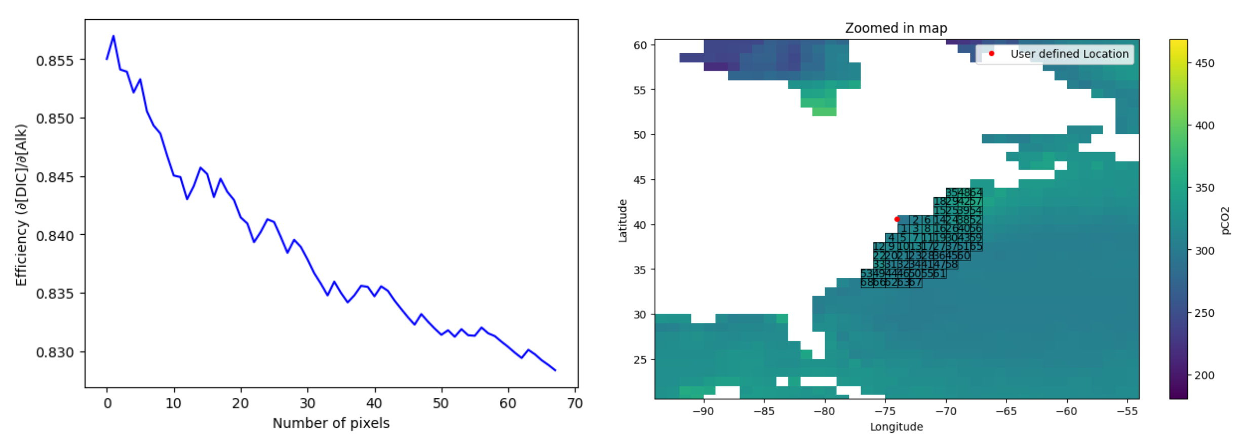
Figure 3 Sensitivity of the ocean retention factor to the number of pixels of data averaged (left), and location of nearest pixels that were used (right).
11.0
Relevant Works
Footnotes
-
Renforth, P., & Henderson, G. (2017). Assessing ocean alkalinity for carbon sequestration. Reviews of Geophysics, 55(3), 636–674. https://doi.org/10.1002/2016RG000533 ↩
-
Ringham, M. C., Hirtle, N., Shaw, C., Lu, X., Herndon, J., Carter, B. R., and Eisaman, M. D. (2024). An assessment of ocean alkalinity enhancement using aqueous hydroxides: kinetics, efficiency, and precipitation thresholds. Biogeosciences, 21, 3551–3570. https://doi.org/10.5194/bg-21-3551-2024 ↩
-
Moras, C. A., Bach, L. T., Cyronak, T., Joannes-Boyau, R., & Schulz, K. G. (2022). Ocean alkalinity enhancement – avoiding runaway CaCO3 precipitation during quick and hydrated lime dissolution. Biogeosciences, 19(15), 3537–3557. https://doi.org/10.5194/bg-19-3537-2022 ↩
-
Suitner, N., Faucher, G., Lim, C., Schneider, J., Moras, C. A., Riebesell, U., & Hartmann, J. (2024). Ocean alkalinity enhancement approaches and the predictability of runaway precipitation processes. Biogeosciences, 21(20), 4587–4604. https://doi.org/10.5194/bg-21-4587-2024 ↩
-
Renforth, P., & Henderson, G. (2017). Assessing ocean alkalinity for carbon sequestration. Reviews of Geophysics, 55(3), 636–674. https://doi.org/10.1002/2016RG000533 ↩
-
Raymond, P. A., Zappa, C. J., Butman, D., Bott, T. L., Potter, J., Mulholland, P., Laursen, A. E., McDowell, W. H., & Newbold, D. (2012). Scaling the gas transfer velocity and hydraulic geometry in streams and small rivers. Limnology and Oceanography: Fluids and Environments, 2, 41–53. https://doi.org/10.1215/21573689-1597669 ↩ ↩2
-
Bach, L. T. (2024). The additionality problem of ocean alkalinity enhancement. Biogeosciences, 21(1), 261–277. https://doi.org/10.5194/bg-21-261-2024 ↩
-
Deirmendjian, L. & Abril, G. (2018). Carbon dioxide degassing at the groundwater-stream-atmosphere interface: isotopic equilibration and hydrological mass balance in a sandy watershed. Journal of Hydrology, 558, 129-143. [https://doi.org/10.1016/j.jhydrol.2018.01.003] ↩
-
Hotchkiss, E. R., Hall Jr, R. O., Sponseller, R. A., Butman, D., Klaminder, J., Laudon, H., Rosvall, M., & Karlsson, J. (2015). Sources of and processes controlling CO2 emissions change with the size of streams and rivers. Nature Geoscience, 8, 696-699. [https://doi.org/10.1038/ngeo2507] ↩
-
Raymond, P. A., Hartmann, J., Lauerwald, R., Sobek, S., McDonald, C., Hoover, M., Butman, D., Striegl, R., Mayorga, E., Humborg, C., Kortelainen, P., Dürr, H., Meybeck, M., Ciais, P., & Guth, P. (2013). Global carbon dioxide emissions from inland waters. Nature, 503, 355–359. [https://doi.org/10.1038/nature12760] ↩ ↩2
-
Martinsen, K. T., Kragh, T., & Sand-Jensen, K. (2020). Carbon dioxide partial pressure and emission throughout the Scandinavian stream network. Global Biogeochemical Cycles, 34(12). [https://doi.org/10.1029/2020GB006703] ↩
-
Bertagni, M. B., & Porporato, A. (2022). The carbon-capture efficiency of natural water alkalinization: Implications for enhanced weathering. Science of The Total Environment, 838, 156524. [https://doi.org/10.1016/j.scitotenv.2022.156524] ↩ ↩2
-
Knapp, W. J., & Tipper, E. T. (2022). The efficacy of enhancing carbonate weathering for carbon dioxide sequestration. Frontiers in Climate, 4, Article 928215. [https://doi.org/10.3389/fclim.2022.928215] ↩
-
Szramek, K., & Walter, L. M. (2004). Impact of carbonate precipitation on riverine inorganic carbon mass transport from a mid-continent, forested watershed. Aquatic Geochemistry, 10, 99–137. https://doi.org/10.1023/B:AQUA.0000038960.63501.5b ↩
-
Neal, C. (2002). Calcite saturation in eastern UK rivers. Science of the Total Environment, 282-283, 311–326. https://doi.org/10.1016/s0048-9697(01)00921-4 ↩
-
Zhang, S., Planavsky, N. J., Katchinoff, J., Raymond, P. A., Kanzaki, Y., Reershemius, T., & Reinhard, C. T. (2022). River chemistry constraints on the carbon capture potential of surficial enhanced rock weathering. Limnology and Oceanography, 67(S2), S148–S157. [https://doi.org/10.1002/lno.12244] ↩ ↩2
-
Zhang, S., Reinhard, C. T., Liu, S., Kanzaki, Y., & Planavsky, N. J. (2025). A framework for modeling carbon loss from rivers following terrestrial enhanced weathering. Environmental Research Letters, 20(2), 024014. [https://doi.org/10.1088/1748-9326/ada398] ↩ ↩2
-
Liu, S., Kuhn, C., Amatulli, G., Aho, K., Butman, D. E., Allen, G. H., Lin, P., Pan, M., Yamazaki, D., Brinkerhoff, C., Gleason, C. J., Xia, X., & Raymond, P. A. (2022). The importance of hydrology in routing terrestrial carbon to the atmosphere via global streams and rivers. Proceedings of the National Academy of Sciences, 119(28), e2106322119. https://doi.org/10.1073/pnas.2106322119 ↩ ↩2
-
Wurgaft, E., Wang, Z. A., Churchill, J. H., Dellapenna, T., Song, S., Du, J., et al. (2021). Particle triggered reactions as an important mechanism of alkalinity and inorganic carbon removal in river plumes. Geophysical Research Letters, 48, e2021GL093178. https://doi.org/10.1029/2021GL093178 ↩ ↩2
-
Ringham, M. C., Hirtle, N., Shaw, C., Lu, X., Herndon, J., Carter, B. R., and Eisaman, M. D. (2024). An assessment of ocean alkalinity enhancement using aqueous hydroxides: kinetics, efficiency, and precipitation thresholds, Biogeosciences, 21, 3551–3570, https://doi.org/10.5194/bg-21-3551-2024 ↩ ↩2 ↩3 ↩4
-
Schulz, K. G., Bach, L. T., and Dickson, A. G. (2023). Seawater carbonate chemistry considerations for ocean alkalinity enhancement research: theory, measurements, and calculations. State of the Planet, 2-oae2023, 2, https://doi.org/10.5194/sp-2-oae2023-2-2023. ↩ ↩2
-
Moras, C. A., Bach, L. T., Cyronak, T., Joannes-Boyau, R., and Schulz, K. G. (2022) Ocean alkalinity enhancement – avoiding runaway CaCO3 precipitation during quick and hydrated lime dissolution, Biogeosciences, 19, 3537–3557, https://doi.org/10.5194/bg-19-3537-2022 ↩ ↩2 ↩3 ↩4
-
Iglesias-Rodríguez, M. D., Rickaby, R. E. M., Singh, A., and Gately, J. A. (2023). Laboratory experiments in ocean alkalinity enhancement research, in: Guide to Best Practices in Ocean Alkalinity Enhancement Research, Copernicus Publications, State Planet, 2-oae2023, 5, https://doi.org/10.5194/sp-2-oae2023-5-2023 ↩ ↩2
-
He and Tyka (2023) Limits and CO2 equilibration of near-coast alkalinity enhancement. Biogeosciences, 20, 27–43. https://doi.org/10.5194/bg-20-27-2023 ↩ ↩2
-
Bach, L. T. (2024) The additionality problem of Ocean Alkalinity Enhancement. Biogeosciences, 21, 261–277. https://bg.copernicus.org/articles/21/261/2024/ ↩ ↩2 ↩3
-
Harrington, K. J., Hilton, R. G., & Henderson, G. M. (2023). Implications of the riverine response to enhanced weathering for CO₂ removal in the UK. Applied Geochemistry, 152, 105643. [https://doi.org/10.1016/j.apgeochem.2023.105643] ↩
-
Kantzas, E. P., Val Martin, M., Lomas, M. R., Eufrasio, R. M., Renforth, P., Lewis, A. L., ... & Beerling, D. J. (2022). Substantial carbon drawdown potential from enhanced rock weathering in the United Kingdom. Nature Geoscience, 15(5), 382-389. [https://doi.org/10.1038/s41561-022-00925-2] ↩
-
Beerling, D. J., Kantzas, E. P., Lomas, M. R., Wade, P., Eufrasio, R. M., Renforth, P., ... & Banwart, S. A. (2020). Potential for large-scale CO2 removal via enhanced rock weathering with croplands. Nature, 583(7815), 242-248. [https://doi.org/10.1038/s41586-020-2448-9] ↩ ↩2
-
Kanzaki, Y., Planavsky, N. J., & Reinhard, C. T. (2023). New estimates of the storage permanence and ocean co-benefits of enhanced rock weathering. PNAS nexus, 2(4). [https://doi.org/10.1093/pnasnexus/pgad059] ↩ ↩2 ↩3 ↩4
-
Humphreys, M. P., Lewis, E. R., Sharp, J. D., & Pierrot, D. (2022). PyCO2SYS v1.8: marine carbonate system calculations in Python. Geoscientific Model Development, 15, 15–43. [https://doi.org/10.5194/gmd-15-15-2022] ↩
-
Humphreys, M. P., Daniels, C. J., Wolf-Gladrow, D. A., Tyrrell, T., & Achterberg, E. P. (2018). On the influence of marine biogeochemical processes over CO₂ exchange between the atmosphere and ocean. Marine Chemistry, 199, 1–11. [https://doi.org/10.1016/j.marchem.2017.12.006] ↩
-
Wilkinson, M., Dumontier, M., Aalbersberg, I. et al. (2016). The FAIR Guiding Principles for scientific data management and stewardship. Scientific Data, 3, 160018. https://doi.org/10.1038/sdata.2016.18 ↩
-
Mu, L., Palter, J. B., & Wang, H. (2023). Considerations for hypothetical carbon dioxide removal via alkalinity addition in the Amazon River watershed. Biogeosciences, 20(10), 1963-1977. [https://doi.org/10.5194/bg-20-1963-2023] ↩
-
Suitner, N., Faucher, G., Lim, C., Schneider, J., Moras, C. A., Riebesell, U., and Hartmann, J. (2024). Ocean alkalinity enhancement approaches and the predictability of runaway precipitation processes: results of an experimental study to determine critical alkalinity ranges for safe and sustainable application scenarios, Biogeosciences, 21, 4587–4604, [https://doi.org/10.5194/bg-21-4587-2024] ↩
-
Jokiel, P. L. (2011). The reef coral two compartment proton flux model: A new approach relating tissue-level physiological processes to gross corallum morphology. Journal of Experimental Marine Biology and Ecology, 409(1–2), 1–12. [https://doi.org/10.1016/j.jembe.2011.10.008] ↩
-
Bach, L. T. (2015). Reconsidering the role of carbonate ion concentration in calcification by marine organisms. Biogeosciences, 12(16), 4939-4951 [https://doi.org/10.5194/bg-12-4939-2015] ↩
-
Monteiro, F. M., Bach, L. T., Brownlee, C., Bown, P., Rickaby, R. E., Poulton, A. J., ... & Ridgwell, A. (2016). Why marine phytoplankton calcify. Science Advances, 2(7). [https://doi.org/10.1126/sciadv.1501822] ↩ ↩2
-
Bach, L.T., Gill, S.J., Rickaby R.E.M., et. al. (2019) CO₂ Removal With Enhanced Weathering and Ocean Alkalinity Enhancement: Potential Risks and Co-benefits for Marine Pelagic Ecosystems. Frontiers in Climate. 1:7. [https://doi.org/10.3389/fclim.2019.00007] ↩
-
Langer, G., Geisen, M., Baumann, K. H., Kläs, J., Riebesell, U., Thoms, S., & Young, J. R. (2006). Species‐specific responses of calcifying algae to changing seawater carbonate chemistry. Geochemistry, geophysics, geosystems, 7(9). [https://doi.org/10.1029/2005GC001227] ↩
-
Renforth, P. (2019) The negative emission potential of alkaline materials. Nature Communications, 10, 1401. [https://doi.org/10.1038/s41467-019-09475-5] ↩
-
Hay, B. J. (1988). Sediment accumulation in the central western Black Sea over the past 5100 years. Paleoceanography, 3(4), 491-508. [https://doi.org/10.1029/PA003i004p00491] ↩
-
Kopelevich, O., Burenkov, V., Sheberstov, S., Vazyulya, S., Kravchishina, M., Pautova, L., ... & Grigoriev, A. (2014). Satellite monitoring of coccolithophore blooms in the Black Sea from ocean color data. Remote sensing of environment, 146, 113-123. [https://doi.org/ 10.1016/j.rse.2013.09.009] ↩
-
Bach, L. T., Mackinder, L. C., Schulz, K. G., Wheeler, G., Schroeder, D. C., Brownlee, C., & Riebesell, U. (2013). Dissecting the impact of CO2 and pH on the mechanisms of photosynthesis and calcification in the coccolithophore Emiliania huxleyi. New Phytologist, 199(1), 121-134. [https://doi.org/10.1111/nph.12225] ↩
-
Bach, L. T., Riebesell, U., Gutowska, M. A., Federwisch, L., & Schulz, K. G. (2015). A unifying concept of coccolithophore sensitivity to changing carbonate chemistry embedded in an ecological framework. Progress in Oceanography, 135, 125-138. [https://doi.org/10.1016/j.pocean.2015.04.012] ↩
-
Bednaršek, N., Pelletier, G., van de Mortel, H., García-Reyes, M., Feely, R., & Dickson, A. (2024). Unifying framework for assessing sensitivity for marine calcifiers to ocean alkalinity enhancement identifies winners, losers and biological thresholds–importance of caution with precautionary principle. EGUsphere, 2024, 1-37 [https://doi.org/10.5194/egusphere‑2024‑947] ↩
-
Gately, J. A., Kim, S. M., Jin, B., Brzezinski, M. A., & Iglesias-Rodriguez, M. D. (2023). Coccolithophores and diatoms resilient to ocean alkalinity enhancement: A glimpse of hope?. Science Advances, 9(24), eadg6066. [https://doi.org/10.1126/sciadv.adg6066] ↩
-
Jia, M., Jacques, D., Gerard, F., Su, D., Mayer, K. U., & Šimůnek, J. (2021). A benchmark for soil organic matter degradation under variably saturated flow conditions. Computational Geosciences, 25(4), 1359–1377. [https://doi.org/10.1007/s10596-021-10099-x] ↩
-
Jia, M., Lapen, D. R., Su, D., & Mayer, K. U. (2025). Multi-domain reactive transport modeling of GHG emissions from macroporous agricultural soils with a focus on N₂O hotspots and hot moments. Water Resources Research, 61(11), e2025WR040588. [https://doi.org/10.1029/2025WR040588] ↩
-
Kelland, M. E., Wade, P. W., Lewis, A. L., Taylor, L. L., Sarkar, B., Andrews, M. G., Lomas, M. R., Cotton, T. E. A., Kemp, S. J., James, R. H., Pearce, C. R., Hartley, S. E., Hodson, M. E., Leake, J. R., Banwart, S. A., & Beerling, D. J. (2020). Increased yield and CO₂ sequestration potential with the C₄ cereal Sorghum bicolor cultivated in basaltic rock dust‑amended agricultural soil. Global Change Biology, 26(6), 3658–3676. [https://doi.org/10.1111/gcb.15089] ↩
-
Lewis, A. L., Sarkar, B., Wade, P., Kemp, S. J., Hodson, M. E., Taylor, L. L., Yeong, K. L., Davies, K., Nelson, P. N., Bird, M. I., Kantola, I. B., Masters, M. D., DeLucia, E., Leake, J. R., Banwart, S. A., & Beerling, D. J. (2021). Effects of mineralogy, chemistry and physical properties of basalts on carbon capture potential and plant‑nutrient element release via enhanced weathering. Applied Geochemistry, 132, Article 105023. [https://doi.org/10.1016/j.apgeochem.2021.105023] ↩
-
Vienne, A., Poblador, S., Portillo‑Estrada, M., Hartmann, J., Ijiehon, S., Wade, P., & Vicca, S. (2022). Enhanced weathering using basalt rock powder: Carbon sequestration, co‑benefits and risks in a mesocosm study with Solanum tuberosum. Frontiers in Climate, 4, Article 869456. [https://doi.org/10.3389/fclim.2022.869456] ↩
-
Kanzaki, Y., Zhang, S., Planavsky, N. J., & Reinhard, C. T. (2022). Soil Cycles of Elements simulator for Predicting TERrestrial regulation of greenhouse gases: SCEPTER v0.9. Geoscientific Model Development, 15, 4959–4990. [https://doi.org/10.5194/gmd‑15‑4959‑2022] ↩
-
Baek, S. H., Lora, J. M., Planavsky, N. J., Kanzaki, Y., Reinhard, C. T., & Zhang, S. (2023). Impacts of climate on the global capacity for enhanced rock weathering on croplands. Earth’s Future, 11(1), Article e2023EF003698. [https://doi.org/10.1029/2023EF003698] ↩
Contributors

Jing He, Ph.D.

Jennifer Yin, Ph.D.

Sophie Gill, Ph.D.

Xueya Lu, Ph.D.
Isometric
River and Ocean Losses © 2026 Isometric HQ Ltd is licensed under CC BY-NC-ND 4.0