Contents
1.0
Summary
This Protocol provides the requirements and procedures for the calculation of net carbon dioxide equivalent (CO2e) removal from the atmosphere via enhanced weathering (EW) in agricultural settings. Agricultural EW is considered a subcategory of EW approaches.
Silicate weathering naturally sequesters approximately 0.1-0.3 Gt of CO2 per year1 ,2 ,3 and is thus a critical feedback mechanism in global climate regulation on geologic timescales. In this process, atmospheric CO2 dissolved in surface water reacts with silicate rocks and is converted to dissolved inorganic carbon or carbonate minerals, both of which constitute stable sinks for CO2 on geologic timescales4 ,5. Natural weathering can be accelerated by applying crushed silicate rock to agricultural land, where the increased reactive surface area of the rock and damp conditions in the soil lead to elevated reaction rates. Alkaline species produced through weathering reactions allow for the increased storage of CO2 in the aqueous phase, typically as dissolved bicarbonate. This dissolved inorganic carbon is eventually exported to the ocean where it can be stably stored for millennia 6. This process is known as enhanced weathering and has been proposed as an effective natural Carbon Dioxide Removal (CDR) technique, in accordance with the IPCC7, to mitigate potential impacts of anthropogenic climate change8. Given that cropland covers approximately 38% of land surface on Earth, EW in agricultural settings has large scalability potential with relatively small changes in farm management. Scalability is aided by existing infrastructure of rock spreading as a soil amendment. Current estimates suggest that EW in cropland has the capacity to remove on the order of 1-2 Gt of CO2 per year8. In addition to CO2 removal, EW can potentially provide co-benefits to farmers in the form of increased crop yield and resiliency9,10, as well as replenishment of soil nutrients11,12 and reduction of nitrogen loss9,13.
This Protocol accounts for the quantification of the gross amount of CO2 removed via agricultural EW, as well as all cradle-to-grave life-cycle Greenhouse Gas (GHG) emissions associated with the process.
This Protocol is developed to adhere to the requirements of ISO 14064-2: 2019 -- Greenhouse Gases -- Part 2: Specification with guidance at the project level for quantification, monitoring, and reporting of greenhouse gas emission reductions or removal enhancements. The Protocol ensures:
-
consistent, accurate procedures are used to measure and monitor all aspects of the EW process required to enable accurate accounting of net CO2e removals
-
consistent system boundaries and calculations are utilized to quantify net CO2e removal for agricultural EW projects
-
requirements are met to ensure the CO2e removals are additional
-
evidence is provided and verified by independent third parties to support all net CO2e removal claims
1.1
Co-benefits and Opportunities
In addition to CO2 removal, dissolution of silicate rocks in agricultural settings may provide co-benefits through the addition of nutrients, alkalinity and silica in soils. Potential co-benefits include:
-
Combating soil acidification through addition of alkalinity9
-
Enhanced crop resistance to common pests and disease17,18,19
-
Increased crop resilience to drought20
-
Decreased nitrogen loss, leading to reductions in fertilizer use, eutrophication and nitrous oxide emissions18, 13
Increased soil nutrients and crop resilience by EW can lead to increased yields, which may help to alleviate global food insecurity if deployed at scale. EW also has the potential to further mitigate emissions via reduction of nitrous oxide fluxes in cropland, which currently represent 50-80% of global anthropogenic N2O emissions13.
2.0
Sources and Reference Standards & Methodologies
This protocol mainly utilizes and is intended to be compliant with the following standards and protocols:
-
(e.g., ISO, EN, 14064-2: 2019 - Greenhouse Gases - Part 2: Specification with guidance at the project level for quantification, monitoring, and reporting of greenhouse gas emission reductions or removal enhancements
Additional reference standards that inform the requirements and overall practices incorporated in this Protocol include:
-
ISO 14064-3: 2019 - Greenhouse Gases - Part 3: Specification with Guidance for the verification and validation of greenhouse gas statements
-
ISO 14040: 2006 - Environmental Management - Lifecycle Assessment - Principles & Framework
-
ISO 14044: 2006 - Environmental Management - Lifecycle Assessment - Requirements & Guidelines
Additional standards, methodologies and protocols that were reviewed, referenced or for which attempts were made to align with or leverage during development of this Protocol include:
-
Global Rock C-sink, Guidelines for the Certification of Carbon Sinks created by Enhanced Rock Weathering in Croplands, v0.9, Carbon Standards International, October 2022.
-
Enhanced Rock Weathering Methodology, PuroEarth, 2022
-
Criteria for High-Quality Carbon Dioxide Removal, Carbon Direct, Microsoft, 2023
-
BS EN 15978:2011 Sustainability of construction works - Assessment of environmental performance of buildings - Calculation method
3.0
Future Versions
This Protocol was developed based on the current state of the art, publicly available science regarding EW in agriculture. Because EW is a novel CDR approach, with limited published literature, this Protocol incorporates requirements that may be more stringent than some current relevant regulations or other protocols related to EW for CDR.
Future versions of this Protocol may be altered, particularly regarding requirements for demonstrating durability of EW, as the stability of CO2 captured by EW from feedstock dissolution in agricultural soils becomes well demonstrated and documented; reversal risks are proven to be limited; and the overall body of knowledge and data regarding all processes, from feedstock supply to conversion and to permanent storage, is significantly increased.
4.0
Applicability
This Protocol applies to projects or processes which:
-
utilize crushed rock or mineral feedstock applied to agricultural land to capture CO2
-
rock or mineral feedstock is defined as silicate rock containing alkaline earth and alkali metals (i.e. Ca, Mg, K, and Na), applied in sufficient quantities to agricultural land to convert CO2 to aqueous bicarbonate
-
agricultural land includes all arable land and permanent cropland, as defined by the United Nations Food and Agriculture Organization (FAO), including row cropland and pastureland.
-
-
export alkalinity generated through weathering reactions from soils to the ocean via riverine transport (Isometric will address alternative drainage situations in future versions of this Protocol)
This Protocol applies to projects and associated operations that meet all of the following project conditions:
-
the project provides a net-negative CO2e impact (net CO2e removal) as calculated in the GHG Statement, in compliance with Section 7.
-
the project does not disproportionately harm underserved or marginalized communities, in compliance with Section 3.7 of the Isometric Standard and Section 5 of this Protocol.
-
the project is considered additional, in accordance with the requirements of Section 6.4.
-
the project provides long duration storage (>1000 year estimated) of CO2 in seawater and/or soil.
Projects that are explicitly NOT eligible include the following:
-
projects that apply rock or mineral feedstock in non-agricultural settings
-
projects that utilize non-silicate feedstock
-
projects that lead to a sustained net decrease on crop yields
As previously stated, per the UN FAO definition of permanent and arable crop land, meadows and pastureland are eligible for EW projects. This Protocol will refer to monitoring requirements specific to row cropland, such as monitoring crop yield, health, and resiliency. Such measurements may not be applicable to projects taking place on pastureland and therefore may not be required in the Project Design Document (PDD). Justifications to omit measurements in such instances are allowable in the PDD.
5.1
Overarching Principles
Credits issued under Isometric's Enhanced Weathering Protocol are contingent on the implementation, transparent reporting and independent verification of comprehensive safeguards. These safeguards encompass a wide range of considerations, including environmental protection, social equity, community engagement and respect for cultural values. The process mandates that safeguard plans be incorporated into all major project phases, with detailed reports made accessible to stakeholders. Adherence to and verification of environmental and social safeguards, in accordance with Section 3.7 of the Isometric Standard, is a condition for all crediting projects.
5.1.1
Environmental Impact Mitigation Strategies
Ongoing environmental assessment must be completed in accordance with the Isometric Standard to identify potential risks, followed by the development of tailored mitigation plans by subject matter experts where necessary. Project Proponents must first strive to avoid negative environmental impacts. In cases where adverse environmental effects take place, the Project Proponent must develop plans to minimize and rectify them. For example, this could include measures such as employing pollution control technologies. Effective implementation of these measures must also be accompanied by a robust monitoring plan to ensure efficacy. Project Proponents must demonstrate active stakeholder engagement throughout this process, in accordance with Section 3.5 of the Isometric Standard. All mitigation strategies must align with local and international environmental laws and contribute to sustainable project outcomes.
5.2
Environmental Safeguards
Enhanced Weathering of rock or mineral feedstock may be associated with the release of metals such as nickel (Ni) and chromium (Cr), which may pose an environmental risk. To prevent or mitigate such risks, the Project Proponent must take the following measures:
- Comprehensive analyses must be conducted in accordance with Isometric's Rock and Mineral Feedstock Characterization Module. Project Proponents should select rock or mineral feedstocks that minimize the risk of soil and groundwater contamination.
- A robust monitoring system must be established to regularly check for potentially harmful metals in soil and groundwater. This will likely involve periodic sampling and analyses alongside field monitoring for removals. The concentration of metals in soil and water must not exceed the limits established by the local authority where the project is located. In the absence of local regulations, the Project Proponent must adhere to standards set by the European Union (EU), the World Health Organization (WHO) or the United States Environmental Protection Agency (US EPA). Justification behind the regulatory body selection must be provided in the PDD.
- If pre-existing heavy metal concentrations exceed applicable regulatory limits or guidance (as identified in the baseline scenario), the Project may still be considered for crediting against this Protocol. This is contingent on the Project Proponent providing evidence of existing elevated metal concentrations. To qualify, the Project must undertake specific remediation strategies to mitigate the contamination. These strategies could include altering the variety or quantity of feedstock used, implementing soil amendments or introducing phytoremediation practices using plants adept at absorbing heavy metals. It is important to note, however, that any project with pre-existing elevated heavy metal concentrations which further aggravates soil contamination, will not meet the criteria for this Protocol.
5.3.1
Food Supply and Agricultural Impacts
Maintaining agricultural productivity is critical to the environmental and social sustainability of EW projects. The Project Proponent must document how the project will monitor agricultural productivity and soil quality, including which productivity and soil characteristics will be tested and the frequency of testing. If justified, the Project Proponent may use proxy variables in lieu of direct testing or measurement. If productivity or soil quality are demonstrated or anticipated to be adversely affected, the Project Proponent must complete the following:
- The Project Proponent must collaborate with land managers or owners to implement soil management practices that maintain or enhance soil quality. Examples of such practices include regenerative agriculture, diversifying crop rotation, utilizing cover crops, etc.
- The Project Proponent must provide technical support, training and resources to help farmers adapt to any changes in soil conditions due to EW. This support could include advice on changes to soil amendments and sustainable farming practices.
5.4
Monitoring and Adaptive Management
All environmental and social safeguards will be verified to be implemented at all locations in the EW process, including at the feedstock source, transportation, and distribution sites. The Project Proponent must regularly assess the combined environmental impact of EW, which includes (but is not limited to) heavy metal concentrations in crops and groundwater. This may involve collecting data on soil and water quality, biodiversity indicators and agricultural productivity. All data indicators, data collection protocols and data interpretation must be written or performed by subject matter experts. The Project Proponent must use the collected data to inform ongoing management of EW practices. This data must be shared with the public through Isometric's platform, in accordance with Section 6.6 of this Protocol. The Project Proponent must be prepared to adjust the EW strategy based on monitoring results and feedback from environmental studies and community engagement.
6.0
Relation to the Isometric Standard
The following topics are covered briefly in this Protocol due to their inclusion in the Isometric Standard, which governs all Isometric Protocols. See in-text references to the Isometric Standard for further guidance.
6.1
Project Design Document
For each specific project to be evaluated under this Protocol, the Project Proponent must document Project characteristics in a Project Design Document (PDD) as outlined in Section 3.2 of the Isometric Standard. The PDD will form the basis for project verification and evaluation in accordance with this Protocol, and must include consideration of processes unique to each agricultural EW project such as:
-
detailed feedstock characterization (see Section 8)
-
geographical designations of control plot(s) (see Section 9.3.1)
-
description of measurement methods for all required analyses, cross-referenced with relevant standards where applicable
-
description of any geochemical models used to quantify processes relevant to the calculation of CO2 removal that are not directly measurable (see Section 7.4.1.1)
-
a comprehensive sampling plan following Section 9, including climatic monitoring and field management plan
6.2
Verification and Validation
Projects must be validated and project GHG Statement (net CO2e removal) verified by an independent third party consistent with the requirements described in this Protocol as well as in Section 4 of the Isometric Standard.
The Validation and Verification Body (VVB) must consider following requisite components:
- Validate that feedstock adheres to the requirements listed in the Rock and Mineral Feedstock Characterization Module.
- Verify that the quantification approach and monitoring plan adheres to requirements of Section 7, including demonstration of required records.
- Verify that the Environmental & Social Safeguards outlined in Section 5 are met.
- Verify that the project is compliant with requirements outlined in the Isometric Standard.
6.2.1
Verification Materiality
The threshold for Materiality, considering the totality of all omissions, errors and mis-statements, is 5%, in accordance with Section 4.3 of the Isometric Standard.
Verifiers should also verify the documentation of uncertainty of the GHG Statement as required by Section 2.5.7 of the Isometric Standard. Qualitative Materiality issues may also be identified and documented, such as21:
-
control issues that erode the verifier's confidence in the reported data
-
poorly managed documented information
-
difficulty in locating requested information
-
noncompliance with regulations indirectly related to GHG emissions, removals or storage
6.2.2
Site Visits
Project validation and verification must incorporate site visits to project facilities, namely agricultural fields being used as control, treatment and deployment plots, in accordance with the requirements of ISO 14064-3, 6.1.4.2. This is to include, at a minimum, site visits during validation and initial verification to the project site(s). Validators should, whenever possible, observe project operation to ensure full documentation of process inputs and outputs through visual observation.
A site visit must occur at least once every 2 years at each control, treatment and deployment plot.
6.2.3
Verifier Qualifications & Requirements
Verifiers and validators must comply with the requirements defined in Section 4 of the Isometric Standard. In addition, teams shall maintain and demonstrate expertise associated with the specific technologies of interest, including soil sampling, analysis and data processing.
6.3
Ownership
CDR via EW in agriculture is often a result of a multi-step process (such as quarrying, transporting and spreading of rock), with activities in each step managed and operated by a different operator, company or owner. When there are multiple parties involved in the process, and to avoid double counting of CO2e removals, a single Project Proponent must be specified contractually as the sole owner of the Credits. Contracts must comply with all requirements defined in Section 3.1 of the Isometric Standard.
6.4
Additionality
The GHG Removal Project Proponent shall be able to demonstrate additionality through compliance with Section 2.5.3 of the Isometric Standard. The baseline scenarios and counterfactual utilized to assess additionality must be project-specific, and are described in Sections 7 and 9 of this Protocol.
Additionality determinations should be reviewed and completed at the time of initial verification or whenever project operating conditions change significantly, such as the following:
-
regulatory requirements or other legal obligations for project implementation change or new requirements are implemented
-
project financials indicate Carbon Finance is no longer required, potentially due to, for example:
-
increased tipping fees for waste feedstocks
-
sale of co-products that make the business viable without Carbon Finance
-
reduced rates for capital access
-
Any review and change in the determination of additionality shall not affect the availability of Carbon Finance and Carbon Credits for the current or past Crediting Periods, however, if the review indicates the Project has become non-additional, this shall make the Project ineligible for future Credits22.
6.5
Uncertainty
The uncertainty in the overall estimate of the net CO2e removal as a result of the Project must be accounted for. The total net CO2e removed for a specific Reporting Period, , CO2eRemoval, RP, must be conservatively determined in accordance with the requirements outlined in Section 2.5.7 of the Isometric Standard.
6.5.1
Reporting of Uncertainty
Projects must report a list of all input variables used in the net CO2e removal calculation and their uncertainties, including:
- required measurements in Appendix 2 (e.g., soil and porewater measurements)
- data used to model and estimate riverine losses and marine losses
- emission factors utilized, as published in public and other databases used
- values of measured parameters from process instrumentation, such as truck weights from weigh scales, electricity usage from utility power meters and other similar equipment
- laboratory analyses, including analysis of rock or mineral feedstocks
More detailed uncertainty information should be provided if available, as outlined in Section 2.5.7 of the Isometric Standard.
In addition, a sensitivity analysis that demonstrates the impact of each input parameter's uncertainty on the overall net CO2e removal uncertainty must be provided. Details of the sensitivity analysis method must be provided so that the results can be re-created. Input variables may be omitted if they contribute to a < 1% change in the net CO2e removal.
6.6
Data Sharing
In accordance with the Isometric Standard, all evidence and data related to the underlying quantification of CO₂e removal and environmental and social safeguards monitoring will be available to the public through Isometric's platform. That includes:
- Project Design Document
- GHG Statement
- Measurements taken and supporting documentation, such as calibration certificates
- Emission factors used
- Scientific literature used
- Proof of approval for necessary permits
The Project Proponent can request certain information to be restricted (only available to authorized Buyers, the Registry and VVB) where it is subject to confidentiality. This includes emissions factors from licensed databases. However, all other numerical data produced or used as part of the quantification of net CO₂e removal will be made available.
7.0
Quantification of CO2e Removal
7.1
Systems Boundary & GHG Emission Scope
The scope of this Protocol includes GHG sources, sinks and reservoirs (SSRs) associated with an EW CDR project. A cradle-to-grave GHG Statement must be prepared encompassing the GHG emissions relating to the activities outlined within the system boundary (Figure 1).
Emissions for processes within the system boundary must include all GHG SSRs from the construction or manufacturing of any project-specific physical site and associated equipment; closure and disposal of each site and associated equipment; and operation of each process (including feedstock production, transport, spreading and sampling for MRV) to include embodied emissions of consumables in the process.
Any emissions from sub-processes or process changes that would not have taken place without the CDR project, such as subsequent transportation and refining, must be fully considered in the system boundary. Paired with exclusion of waste input emissions when the criteria are met (see Section 7.1.1), this allows for accurate consideration of additional, incremental emissions induced by the CDR process.
The system boundary must include all SSRs controlled by and related to the project, including but not limited to the SSRs in Figure 1 and Table 1. If any GHG SSRs within Table 1 are deemed not appropriate to include in the system boundary, they may be excluded provided that robust justification and appropriate evidence is provided.
Figure 1. Process flow diagram showing system boundary for EW projects
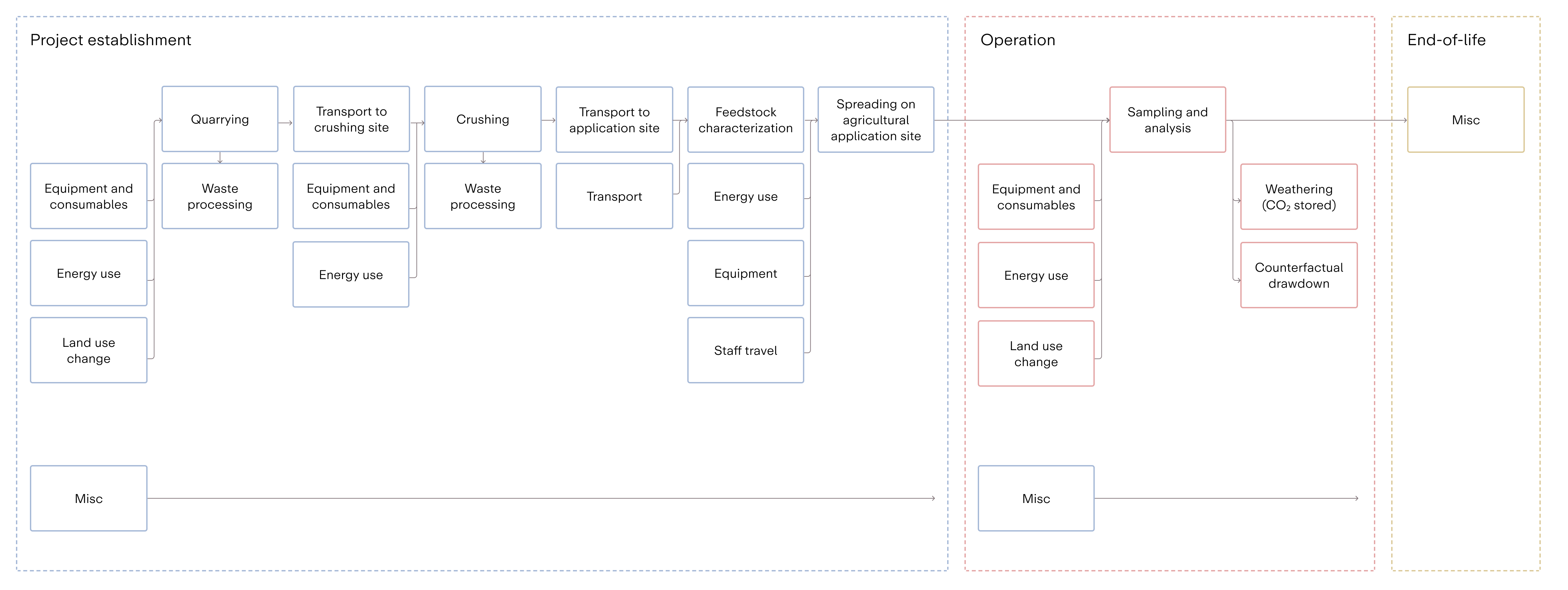
Table 1. Systems boundary and scope of activities to be included for EW projects
| Activity | GHG source, sink or reservoir | GHG | Scope | Timescale of emissions and accounting allocation |
|---|---|---|---|---|
| Establishment of project | Quarrying | All GHGs | Quarrying activities including the following emissions sources:
| Before Reporting Period - must be accounted for in the first Reporting Period or amortized in line with allocation rules (See Section 7.4.3.1) |
| Transport to crushing site | All GHGs | Transporting the feedstock material from the excavation site to the crushing facility | ||
| Crushing and grinding (including additional processing steps such as drying) | All GHGs | Crushing and grinding activities including the following emissions sources:
| ||
| Feedstock transport to application site | All GHGs | Transporting the feedstock material from the quarrying site to the agricultural application site | ||
| Feedstock characterization | All GHGs | Embodied, energy use and transport emissions associated with sampling the feedstock to measure the physical and geochemical characteristics necessary for weathering determinations | ||
| Spreading on agricultural application site | All GHGs | Spreading activities including:
| ||
| Misc. | All GHGs | Any GHG SSR not captured by categories above, for example related to field surveys | ||
| Operation | Sampling and analysis | All GHGs | Sampling and analysis activities, including:
| Over each Reporting Period - must be accounted for in the relevant Reporting Period (See Section 7.4.3.2) |
| CO2 stored | CO₂ | The gross amount of CO2 removed and durably stored from an EW project over a Reporting Period | ||
| Misc. | All GHGs | Any GHG SSR not captured by categories above, for example related to refrigeration for storing soil cores | ||
| End-of-Life | Misc. | All GHGs | Activities post-Reporting Period, for example end-of-life emissions associated with equipment or deconstructing infrastructure | After Reporting Period - must be accounted for in the first Reporting Period or amortized in line with allocation rules (See Section 7.4.4.3) |
The Project Proponent must consider all GHGs associated with SSRs, in alignment with the United States Environmental Protection Agency’s definition of GHGs, which includes: carbon dioxide (CO₂), methane (CH4), nitrous oxide (N2O) and fluorinated gasses such as hydrofluorocarbons (HFCs), perfluorocarbons (PFCs), sulfur hexafluoride (SF6) and nitrogen trifluoride (NF3). For CO2 stored, only CO2 shall be included as part of the quantification. For all other activities all GHGs must be considered. For example, the release of CO2, CH4, and N2O is expected during diesel consumption.
All GHGs must be quantified and converted to CO2e in the GHG Statement using the 100-yr Global Warming Potential (GWP) for the GHG of interest, based on the most recent volume of the IPCC Assessment Report (currently the Sixth Assessment Report).
Miscellaneous GHG emissions are those that cannot be categorized by the GHG SSR categories provided in Table 1. The Project Proponent is responsible for identifying all sources of emissions directly or indirectly related to project activities and must report any outside of the SSR categories identified as miscellaneous emissions.
Emissions associated with a project's impact on activities that fall outside of the system boundary of a project must also be considered. This is covered under Leakage in Section 7.4.3.4.
7.1.1
Exclusions from system boundary
The following are excluded from system boundaries:
7.1.1.1
Ancillary activities
Ancillary activities (such as supplementary research and development activities and corporate administrative activities) that are associated with a project but are not directly or indirectly related to the issuance of Credits can be excluded from the system boundary.
7.1.1.2
Secondary Impacts on GHG emissions
EW may have additional impacts on GHG emissions beyond the scope of this Protocol. For example, there is some evidence that EW in agriculture may have secondary impacts on N2O and CH4 emissions associated with agricultural soils. These potential impacts are not currently included in the conservative GHG accounting framework and will be reviewed as scientific consensus evolves.
Similarly, emissions reductions associated with other processes that could arise as a result of the EW project should not be credited toward the project.
7.1.1.3
Considerations for Waste Input Emissions
Embodied emissions associated with system inputs considered as waste products can be excluded from the accounting of the GHG Statement system boundary of the CDR process if all of the below criteria are met:
- The waste product is fundamentally tied to or is the result of a separate process.
- The separate process was already operating or was likely to continue operating in absence of the CDR process.
- The amount of the waste product used by the CDR project was not already being utilized as a valuable by-product or co-product by another party for non-CDR uses.
- Market leakage emissions are fully considered.
- The separate process has a pathway toward compliance with net-zero emissions.
An example to illustrate this would be crushed residues generated by an operational, profitable mine. If the residues would likely be generated without an EW project as a baseline scenario, and the rest of the criteria above are met, they can be used in the GHG accounting without an emissions burden. However, emissions relating to the processing of these residues, such as screening, drying and transport, should be included in the GHG Statement. The Project Proponent must provide documentation that the above criteria are met in order to omit such emissions from the GHG Statement.
In the case that a relevant separate process would not continue operating or would not begin operating without revenue from waste product valorization, emissions should be allocated to the waste product used in the system boundary. In the case that a waste product from a separate process was already being used as a by-product to serve some other process, emissions generated from the displacement of the supply of the by-product must be considered as part of the Leakage assessment.
7.1.1.4
Considerations for Project Activities Integrated into Existing Practices
In some instances, the EW project activities may be integrated into existing activities, such as rock spreading whilst seeding. Activities that were already occurring and would continue to occur without the EW project may be omitted from the system boundary of the GHG accounting, if evidence that the activity was already occurring and would have continued to occur in the absence of the EW project can be provided.
7.2
Baseline
The baseline scenario for EW projects assumes the activities associated with the EW project do not take place, no new infrastructure is built and business as usual agricultural practices occur.
The counterfactual is the CO2 that would have been removed from the atmosphere and durably stored as a result of natural weathering or pre-existing land practices. This is determined through the use of a control plot, as descibed in Section 7.4.2, with detail on monitoring requirements described in Section 9.3.4.3.
7.3
Net CDR Calculation
7.3.1
Calculation Approach and Reporting Period
EW in agriculture typically consists of an application of a characterized rock or mineral feedstock followed by discrete sampling periods to quantify CO2 removals. Rock or mineral feedstock must be sourced, which may include quarrying, processing (e.g., crushing) and transportation, before it is spread over agricultural land. A combination of soil and aqueous measurements are then used to quantify the total CO2 removals over a period of time.
The Reporting Period for EW represents an interval of time over which removals are calculated and reported for verification. Monitoring of CO2 removals for EW may include a combination of discrete sampling (e.g., soil sampling) and continuous sampling. The equations used to calculate net CO2e removals will pertain to all GHG emissions and CO2 removals occurring over a Reporting Period. In most cases, this Reporting Period will be an interval of time bounded by sampling events.
GHG emission calculations must include all emissions related to the project activities that occur within the Reporting Period. This includes: a) any emissions associated with project establishment allocated to the Reporting Period, b) any emissions that occur within the Reporting Period, c) any anticipated emissions that would occur after the Reporting Period that have been allocated to the Reporting Period and d) leakage emissions that occur outside of the project boundary as a result of induced market changes that are associated with the Reporting Period. Requirements for allocated emissions to Reporting Periods are set out in Section 7.4.3. All allocated emissions must must be accounted for by the Reporting Period in which 50% of total feedstock weathering potential has been realized.
Total net CO2e removal is calculated for each Reporting Period, and is written hereafter as .
7.4
Calculation of CO2eRemoval, RP
Net CO2e removal for EW in agriculture for each Reporting Period, RP, can be calculated as follows. The final net CO2e removal quantification must be conservatively determined, giving high confidence that at a minimum, the estimated amount of CO2e was removed (refer to Section 6.5 for details).
(Equation 1)
Where:
- -- the total net CO2e removal for the Reporting Period, RP, in tonnes of CO2e
- -- the total CO2 removed from the atmosphere and stored as inorganic carbon in the solid or aqueous form in the treatment and deployment (in 3-plot approach) plots for the RP, in tonnes of CO2e
- - the total counterfactual CO2 removed from the atmosphere and stored as inorganic carbon in the solid or aqueous form for the RP, in tonnes of CO2e
- -- the total GHG emissions for the RP, in tonnes of CO2e
Note: Reversals occur after Credits have been issued so are not included in this equation. See Section 9.2 and Section 5.6 of the Isometric Standard for further information.
7.4.1
Calculation of CO2eStored, RP
Type: Ocean storage
The total amount of CO2 stored from an EW project must include the following terms:
(Equation 2)
Where:
- -- CO2 removed from the release of base cations for Reporting Period, RP, in tonnes of CO2e. These base cations may derive from newly weathered rock or mineral feedstock, net dissolution of carbonate minerals over the previous Reporting , or desorption of base cations that had previously come out of solution by surface sorption.
- -- Inorganic carbon lost due to soil column (bio)geochemical processes for the Reporting Period, RP, as well as downstream riverine and marine losses, in tonnes of CO2e. These losses include plant uptake of base cations, secondary silicate mineral formation, carbonate precipitation, non-carbonic acid neutralization, sorption of base cations to cation exchange sites, re-equilibration of the carbonate system in rivers and oceans and any other relevant processes.
In this mass/charge balance approach, we explicitly account for: 1) permanent losses of base cations (and corresponding CO2 removals) that happen after base cations are released from a rock or mineral feedstock through weathering and 2) the possibility that base cations may be temporarily, but not permanently, rendered ineffective for removals. These include both permanent and temporary losses.
Losses considered to be permanent include:
-
Plant biomass uptake of base cations
-
The formation of secondary silicates (e.g., clays)
-
Non-carbonic acid neutralization (e.g., neutralization of acid produced from nitrification of ammonia fertilizers)
-
Degassing due to re-equilibration of the dissolved inorganic carbon system
Losses considered to be temporary include:
-
The formation of carbonate minerals
-
Base cation sorption to cation exchange sites
One particularly consequential aspect of these CO2 removal loss terms is the potential time lag associated with cation sorption. A base cation may undergo many generations of sorption and desorption to cation exchange sites while migrating through the soil column, delaying the CO2 removal effect until that cation is sufficiently deep in the soil column or more permanently transitions to the aqueous phase. There is currently no widely held scientific consensus on the best practices for modeling these cation sorption dynamics.
The sorption of base cations to cation exchange sites will cause re-equilibration of dissolved inorganic carbon species to maintain charge balance, which will result in degassing of CO2 into soil pore space. If this degassing occurs sufficiently deep in the soil column, the resulting transient CO2 may be sufficiently isolated from the atmosphere as to be considered a removal while the cation is still migrating through the soil column.
Here we make the simplifying assumption that once base cations pass through the depth of deepest soil sampling, they can effectively be considered a removal. This Protocol currently recommends this depth to be at minimum 30 centimeters below the surface23,24, but this will likely be refined as theoretical and observational constraints improve. A shallower window of direct soil observations may be used in circumstances where 30 centimeters is not feasible (e.g., water table occurs at a depth less than 30 centimeters, or 30 cm cannot be accessed through conventional sampling methods). Such deviations must be reported and justified in the PDD.
All crediting projects must design a sampling plan that directly measures the initial weathering of rock or mineral feedstock through soil and porewater sampling. Once a statistically significant amount of feedstock weathering has occurred, the Project Proponent may be eligible for Credits. This Protocol allows for two separate determinations of the carbon stored from an EW project: 1) from a combination of soil and porewater measurements and 2) from porewater measurements. Should the Project Proponent choose to measure realized CO2 removal from both determinations for research purposes, the determination used for crediting must be designated in the PDD. If Determination 2 is used for crediting, aqueous phase measurements must be conducted on samples collected from the depth of deepest soil sampling in Determination 1 (i.e., 30 centimeters).
7.4.1.1
Determination 1
The total amount of carbon stored from an EW project can be determined from soil and porewater measurements according to:
(Equation 3)
Where:
- -- CO2 removed from the release of base cations from feedstock for the Reporting Period, RP.
- -- Amount of that is undone by the uptake of base cations by plant biomass for the RP.
- -- Amount of that is undone from the net formation of new carbonate minerals in the soil column for the RP. This will typically lead to a ~50% decrease in the removal efficiency over aqueous phase export.
- -- Amount of that is undone from the formation of new silicate minerals in the soil column for the RP.
- -- Amount of that is undone from the net sorption of base cations to cation exchange sites soil column for Reporting Period RP. We note that, in some cases, this value may be negative, indicating a net release of cations that had accumulated in previous Reporting Periods.
- -- Amount of that is undone from neutralization of acids other than carbonic acid for the RP.
- -- Amount of net in-field that is expected to be released back to the atmosphere due to outgassing in river systems.
- -- Amount of net in-field that is expected to be released back to the atmosphere due to outgassing in the ocean.
All terms have units of tonne CO2e.
Below is an overview of how each term is determined, with more details provided in Section 9.
must be determined from direct geochemical observation of soil in deployment area per Section 9.3.4. A depth of 30 cm is chosen because common tilling depths are unlikely to exceed 30 cm, and 30 cm has become widely used in the EW community to assess feedstock weathering rates. If tillage depth exceeds 30 cm, the minimum sampling depth must be increased to a depth greater than the tillage depth. In such instances, tillage and sampling depth must be reported in the PDD. Shallower sampling may be acceptable for the determination of feedstock weathering if it can be justified based on field management practices and observed depth of feedstock tracer in soil. While shallower sampling is acceptable for determination of initial weathering, 30 cm sample depths should still be used for soil based measurements outlined below (unless alternative sampling depth is justified in PDD). Nearly all emerging methods for determining in-field rely on measuring the abundance of some insoluble elemental or isotopic tracer and its ratio to soluble base cations in the feedstock to determine weathering. This includes measuring the abundance of both insoluble tracer(s) and soluble base cations before and after feedstock application to determine the weathering potential, and measuring the evolution of these two groups of analytes at later time points to determine the gross CO2 removal before accounting for the various losses. The change in the chosen tracer(s) of base cation release must show differences that are statistically significant between the start and the end of the Reporting Period to be eligible for crediting (see Section 9.3.4.2.1). The project must clearly specify all of the following in the PDD:
-
The depth of sampling for determination of weathering rate and a justification if different than 30 cm
-
The insoluble feedstock tracer(s)
-
The soluble base cations being considered for CO2 removal
-
The method(s) used including references to peer reviewed publications and/or standard methodologies
-
Measures being taken to account for or limit interference from alternative sources of base cations (e.g., only using Ca and Mg to determine drawdown to avoid interference from monovalent cations in some fertilizers)
-
The explicit form of the mass balance equation being used to determine the release of base cations from the feedstock over time
-
A pH-dependent unit conversion factor between the aqueous concentration of base cations and CO2 removal
Once the statistical criteria for crediting have been met (see Section 9.3.4.2.1), for the area of interest (may be a treatment or deployment plot if 3-plot approach is used) should be determined by calculating the total CO2 removal in the treatment and deployment areas separately before adding them together.
(Equation 4)
Where:
- -- the change in alkalinity (base cations) in the soil column between the beginning and end of the Reporting Period, as calculated in Equation 17, in eq/kg
- -- the average bulk density of soil in the weathering horizon (typically 30 cm) in area , in kg/m3
- -- the sampling depth, in meters
- -- the area of the treatment or deployment (in 3-plot approach) plot, in m2
- is the pH dependent conversion of alkalinity to carbon stored in the aqueous phase
Additional details on soil based field monitoring are included in Section 9.3.4.
is determined from direct, representative sampling of plant tissues at peak biomass in an area in which feedstock is applied (treatment area if using 3-plot approach) and the control plots (this does not need to be directly measured in the deployment plot if using 3-plot approach). Sampling routines must be identical between areas with and without feedstock. Plant samples must be analyzed for C, N, Na, K, Mg and Ca concentrations (base cations not used for crediting may be omitted from this measurement). Project Proponents are required to cross reference the following standards for their measurement procedures:
-
Total carbon content -- e.g., ISO 10694:1995
-
Total nitrogen content -- e.g., ISO 13878:1998
-
Cation concentrations -- e.g., ISO 17294-1:2024 for ICP-MS or ISO 11885:2007 for ICP-OES
For cation measurements, Project Proponents are required to outline and justify their method for digestion (dissolving sample into liquid phase) of plant material in the PDD.
Sampling plans targeting plant uptake must consider the total amount of new biomass produced over the Reporting Period. Project Proponents are required to include all data and calculations in submitted reports, including information on standards and calibration curves. This data should include total shoot mass, total plant mass and cation concentrations.
The Project Proponent must describe in the PDD how measurements of base cations removed by plant uptake are conservatively extrapolated over the project area for the determination of .
represents the average net change in soil inorganic carbon (SIC) between the start and the end of the Reporting Period. This measurement pertains all soils collected in the observation window, typically 0 to 30 cm, but should also proportionally represent sample fractions if samples are partitioned for determination of initial weathering (e.g., total SIC is determined from a weighted average of 0-10 cm samples and 10-30 cm samples). This Protocol requires that SIC, when measured, is measured via either calcimetry or thermo-gravimetric analysis. This must be quantified using:
-
Calcimetry -- e.g., ISO 23400:2021
-
Thermo-gravimetric analysis -- e.g., ASTM D8474-22
Project Proponents utilizing other determination methods, in consultation with Isometric, must outline and justify these alternative analyses in the PDD.
This value of may be positive, zero or negative. A positive value corresponds to a net increase in soil inorganic carbon, which will result in less CO2 being stored. A negative value corresponds to net dissolution of carbonate minerals, and may lead to net CO2e removal if dissolution is the result of reaction with carbonic acid.
Soil inorganic carbon is typically determined in weight percent (e.g., kg calcium carbonate per kg soil). The corresponding amount of CO2 stored in net new carbonate is determined as follows:
(Equation 5)
(Equation 6)
Where:
- -- the amount of CO2 stored in CaCO3 minerals at time point t, in tonnes.
- -- the mass fraction of a soil sample that is CaCO3, expressed as a percent.
- -- the conversion factor from weight percent to decimal.
- -- a unitless ratio of the molar mass of CO2 to the molar mass of CaCO3.
- -- the average bulk density of soil in area , in kg/m3
- is the sampling depth, in m.
- is the area of the control, treatment, or deployment plot, in m2.
- is the conversion factor from metric tonnes to kilograms.
Some project areas may have soil conditions where carbonate precipitation is not likely and not observed above analytical detection limits (e.g., low pH soils). Project Proponents operating in such areas may omit large scale soil inorganic carbonate measurements from routine monitoring with adequate justification in the PDD. In such instances, Project Proponents must conduct smaller scale measurements of soil inorganic carbon with each major sampling event to demonstrate that these assumptions still hold. If local geochemical conditions change over the course of a project and lead to measurable soil carbonate mineral accumulation, soil inorganic carbonate measurements must be reinstated at the same density as other primary soil measurements.
is the average net change in silicate mineral (e.g., clay mineral) content between the start and end of the Reporting Period. There is no widely accepted and operationally feasible quantitative method for determining modest changes in secondary silicate mineral content in soils; clay content of soils is typically expressed as a percentage of clay-sized particles, and mineralogy is determined by x-ray diffraction. Thus, detection of secondary clay formation requires either significant enough clay formation to shift the percentage of clay-sized particles in the soil column or quantitative formation of clay mineralogies that are distinct from the initial assemblage (unlikely for modest pH change in soils with similar moisture retention; see Wilson (1999) for an overview of the parameters controlling clay formation in soil)25. We have included this term for completeness, but we will not explicitly require measurement of this parameter at this time.
is determined by measuring any change in adsorbed base cations over the Reporting Period. Typically, this is determined using the difference in the product of cation exchange capacity and base cation saturation between the start and end of the Reporting Period. A positive value corresponds to a net increase in base cations sorbed to cation exchange sites, leading to outgassing of dissolved CO2. Conversely, a negative value corresponds to a net decrease in base cations sorbed, leading to CO2 removal. Cation exchange capacity measurements should comply with ISO 11260:2018, ISO 23470:2018 or the Chapman method. Quantification of base saturation should comply with ISO 11260:2018. Some agronomic soil testing facilities may use regionally specific methodologies that deviate from the standards listed above. Such methodologies are generally permissible, but require approval by Isometric. Such alternative methods must be approved by Isometric and justified in the PDD.
may be determined using direct measurements of anions in porewaters, an approximation based on soil pH and pCO2 (see Dietzen et al., 2023) or a conservative estimate based on documented fertilizer application.
If direct measurement of anions is used, samples must be collected at or below the depth to which weathering is being monitored (typically 30 cm). Major anions should include NO3-, PO43-, Cl-, SO42- and any others that may be relevant to local land management practices and the feedstock being used. Measurement methods must comply with ISO 10304-1:2007. Unlike some soil based measurements in this Protocol, aqueous concentration of anions in porewaters will likely be dynamic and vary significantly over a Reporting Period. The Project Proponent must provide details of their sampling plan and describe how the chosen sampling frequency is appropriate for capturing any significant deviation in concentration at the project location.
The Project Proponent must describe in the PDD how site-based observations (e.g., precipitation, irrigation, other climatic variables, etc.) are used to determine the total volume of water infiltrated into the soil, and how discrete anion concentrations are combined with this data to determine the total amount of non-carbonic acid neutralization that occurred over the Reporting Period. Given a known volume of water infiltrated into the soil, can be calculated as:
(Equation 7)
Where:
- -- the charge of the major anion.
- -- the concentration of that anion in solution in ppm.
Dietzen & Rosing (2023) describe a method for determining the proportion of weathering that occurs by reaction with carbonic acid based on carbonate speciation in soil porewater, as determined by measurements of soil pH and CO2 (Dietzen & Rosing 202326, equations 2-9). This formulation can be adapted to determine the proportion of weathering that occurs by reaction with non-carbonic acids using any two components of the carbonic acid system. Project Proponents may elect to account for non-carbonic acid neutralization using this method. Descriptions of the measurement and calculation methods must be provided in the PDD.
Where data is available, Project Proponents may choose to use fertilizer application rates as a proxy for non-carbonic acid weathering. Quantification of non-carbonic acid weathering from fertilizer records may come from:
- Documented fertilizer application rates, assuming that 100% of ammonium applied is nitrified
- Documented fertilizer application rates and measurement of nitrogen use efficiency (plant uptake of nitrogen)
Project Proponents must provide data on fertilizer application rates and calculations of the fraction of feedstock weathering resulting from non-carbonic acid weathering in the PDD. If non-carbonic acid neutralization is accounted for using fertilizer application rates, Project Proponents must provide evidence to justify the assumption that nitric acid is the only significant non-carbonic acid source. This includes measurements of total sulfur in the feedstock and in the soil.
includes all future losses that will occur in river systems downstream of in-field activities. In most cases this will be a modeled result. Models used to estimate riverine losses must use historic river geochemical data to estimate relevant parameters. This may include publicly available datasets or scientific publications. The source of such data must be reported. Models must include explicit consideration of:
-
Formation of new carbonate minerals
-
Outgassing of CO2 due to re-equilibration of DIC system
includes all future losses that will occur after base cations are exported to the ocean. This must include explicit consideration of:
-
Formation of new carbonate minerals
-
Outgassing of CO2 due to re-equilibration of DIC system
7.4.1.1.1
Sample Pooling Prior to Analysis
While this Protocol prescribes a minimum number of soils samples that must be collected for the quantification of removals, it may be appropriate in some cases to pool samples for more resource-intensive analyses (e.g., analysis of trace metal abundance). Solid and liquid phase sample pooling is acceptable in crediting projects, with a maximum of 10 samples pooled per analysis. Samples must be pooled in equal volumes. All sample pooling plans must be approved by Isometric and described in the PDD.
7.4.1.1.2
Aqueous Phase Checks for Determination 1
As scientific consensus on EW continues to develop, redundant measurements are critical to understand carbon removal processes at the field scale. To this end, this Protocol requires that Project Proponents seeking Credits through Determination 1 conduct aqueous check measurements at lower spatial resolution to maximize confidence in calculated CDR. At a minimum, porewaters must be collected at the depth of lowest sampling (typically 30 cm) at a density of 1 porewater sampling device per 50 hectares (total project area). Samples must be collected in control and treatment plots in both the 2- and 3-plot models; aqueous check samples are recommended, but not required, in the deployment plot if using the 3-plot model. Deviation from depth and density requirements may be allowable in consultation with Isometric given site-specific considerations and must be justified in the PDD. Collected aqueous samples must be analyzed for at least two components of the carbonic acid system to calculate bicarbonate concentration; see guidance in Section 9.3.5.1.2. If the mean calculated CDR of aqueous measurements does not fall within the 95% confidence interval of CDR calculated by Equation 3, an audit must be conducted and Project Proponents will work with Isometric to determine a conservative solution.
7.4.1.1.3
Alternative Methods and Approaches for Determination 1
Project Proponents pursuing Determination 1 must consider all terms listed in Equation 3, but alternative methods may be appropriate for rigorous quantification of CDR. For example, some Project Proponents may choose to monitor the loss of alkalinity in a project area by performing full sample digests on soil samples without any pre-processing (e.g. removal of carbonates, extraction of the soil exchangeable fraction). In this instance, weathering, cation sorption, carbonate formation and clay formation will all be integrated into a single measurement. Such deviations may be appropriate and will be considered on a project by project basis. In such cases, the Project Proponent must provide a detailed description of the methods and describe how the chosen analyses map onto the terms in Determination 1 in the PDD.
7.4.1.2
Determination 2
In Determination 2, we make the simplifying assumption that all of the major soil column processes, including the release of base cations from weathering and soil losses, are accounted for in the aqueous geochemistry of water that has infiltrated to some depth. At this time, we are recommending a depth of 30 cm. Therefore, the total amount of carbon stored from an EW project can be determined from porewater measurements in the top 30 cm of soil. Alternatives to 30 cm may be justified for similar reasons described in the previous section. Well-defined catchment waters may be used in place of porewaters where the project area is contained entirely within such well-defined catchments. In instances where catchment waters are used, the Project Proponent must provide supporting documents detailing site-specific hydrogeology.
(Equation 8)
Where:
- -- CO2 removed as determined from the infiltration of carbonate alkalinity to a minimum depth, typically 30 cm, in the Reporting Period, RP.
- -- Amount of net in-field that is expected to be released back to the atmosphere due to outgassing in river systems.
- -- Amount of net in-field that is expected to be released back to the atmosphere due to outgassing in the ocean.
All terms have units of tonne CO2e.
Below is an overview of how each term is determined, with more details provided in Section 9.3.5. It is important to note that, although is not explicitly included in Determination 2, alkalinity may still be taken up by plants below the 30 cm observation window. Project Proponents using Determination 2 for Credits must still consider and quantify plant uptake if roots extend below the depth of porewater sampling.
: This is the integrated amount of CDR as determined from measurements of aqueous phase base cation abundance from water that has infiltrated to a minimum of 30 cm depth. There are two generally accepted approaches for determining aqueous phase alkalinity export: 1) direct measurements of cation and anion concentrations (e.g., ICP) or 2) measurement of at least two carbonic acid system variables in solution. Carbonic acid system measurements may include carbonate alkalinity titration to the CO2 equivalence point, pH, DIC and/or pCO2, followed by calculating the concentration of bicarbonate using the 2-for-6 method. Further guidance is given in Section 9.3.5.1.2.
: See Determination 1
: See Determination 1
7.4.1.2.1
Alternative Methods and Approaches for Determination 2
Project Proponents pursuing Determination 2 must consider all terms listed in Equation 8, but alternative methods may be appropriate for rigorous quantification of CDR. For example, some Project Proponents may choose to directly observe cation and anion concentrations in collected waters. In this instance, weathering and multiple loss terms may be integrated into one result. Such deviations may be appropriate and will be considered on a project by project basis. In such cases, the Project Proponent must provide a detailed description of the methods and describe how the chosen analyses map onto the terms in Determination 2 in the PDD.
7.4.2
Calculation of CO2eCounterfactual, RP
Type: Counterfactual
describes the CO2 that would have been removed from the atmosphere and durably stored in the baseline scenario, as a result of natural weathering or pre-existing land practices. This is calculated using the control plot, which must be subject to business as usual farming practices. The control plot ensures that any removals associated with business as usual agricultural liming are not attributed to EW in agriculture projects. The control plot will serve as the baseline in modelling with respect to measured soil and porewater parameters. The approach used for this accounting, including the feedstock storage location, climatic conditions of the storage location, models used, and/or analyses conducted, must be provided and justified in the PDD.
In addition to counterfactual CO2 related to business as usual farming practices, in some instances it may be appropriate to consider weathering of feedstock that would have occurred without project intervention. For example, if the feedstock used constitutes a waste product that was not mined or quarried specifically for project activities and was stored in open-air conditions, some degree of surfical weathering could be expected over timescales relevant to a project lifetime. Project Proponents using these feedstocks must account for counterfactual weathering if the feedstock does not undergo additional processing prior to deployment. The Isometric Standard defines the durability of a credit as 1000+ years; thus, this is the default assumption for the calculation timescale of counterfactual weathering if no additional information regarding the storage conditions and duration of the feedstock at the mine/quarry site can be provided. If additional information on the conditions and duration of feedstock storage at the feedstock supplier are available, Project Proponents may justify calculating the counterfactual across a time period relevant to the specific mine or quarry from which the feedstock is sourced in the PDD. For example, projects operating in conjunction with active mines may find it appropriate to use the time of mine closure and provide details of the closure plan in the PDD; alternatively, if sufficient documentation exists suggesting that piles of waste materials generated by the feedstock will not be exposed to ambient environmental conditions for a period exceeding a set number of years, the counterfactual may be considered across that time span. It is important to note that studies have shown that the vast majority of weathering in tailings piles occurs in the surface layer that is exposed to the atmosphere, provided that there is no mechanical overturn (citations). For this reason, counterfactual weathering needs to be accounted for in the top meter of the tailings pile.
Where relevant, counterfactual weathering must be calculated by a combination of direct measurements and modeling of the expected weathering rate of feedstock under storage conditions relevant to the source site for either 1000 years or a time period justified in the PDD as described above. Models must be justified by empirical data from subsamples of the feedstock; guidelines for sampling procedures that adequately capture feedstock heterogeneity are described in the Rock and Mineral Feedstock Characterization Module. Models must take into account:
- Feedstock mineralogy (direct measurement)
- Feedstock surface area (direct measurement)
- Baseline carbonation of the tailings pile (direct measurement)
- CDR potential of the tailings pile in the top 1 m (calculated from direct measurements)
- Environmental conditions of the source site (direct measurement or publicly available data), including:
- Temperature
- Average yearly precipitation
- Rainwater pH
- Groundwater pH
- Carbonate saturation
- Permeability (direct measurement or calculated from direct measurement)
- Water saturation (direct measurement or calculated from direct measurement)
- Microbial activity (direct measurement)
The measurements and model used to calculate counterfactual weathering must be provided to Isometric and the VVB. Project Proponents may choose to either assume the total counterfactual as a one-time deduction or to spread the counterfactual deduction across a project lifetime.
is determined using the same equations (Equations 7 and 8) as the previous section for in which all the encompassed terms are determined using a control plot of land as described in Section 9.3.1.
For instances where the Project Proponent has discretion as to which methods can be used to determine a particular weathering or loss term, the methods used must be the same for both the area over which feedstock is applied and the control plot.
7.4.3
Calculation of CO2eEmissions, RP
Type: Emissions
is the total quantity of GHG emissions associated with a Reporting Period . This can be calculated as:
(Equation 9)
Where:
- -- the total GHG emissions for a Reporting Period, RP, in tonnes of CO2e.
- -- the total GHG emissions associated with project establishment for a RP, in tonnes of CO2e.
- -- the total GHG emissions associated with operational processes for a RP, in tonnes of CO2e.
- -- the total GHG emissions that occur after the RP and are allocated to the RP, in tonnes of CO2e, see Section 7.4.3.3.
- -- represents GHG emissions associated with the project’s impact on activities that fall outside of the system boundary of a project, over a given Reporting Period, in tonnes of CO2e, see Section 7.4.3.3.
The following sections set out specific quantification requirements for each variable. It is anticipated that most emissions associated with EW projects will occur during the Calculation of CO2eEstablishment, RP phase.
7.4.3.1
Calculation of CO2eEstablishment, RP
GHG emissions associated with should include all historic emissions incurred as a result of project establishment, including but not limited to the SSRs set out in Table 1.
Project establishment emissions occur from the point of project inception through to after the spreading event has taken place. GHG emissions associated with project establishment may be allocated in one of the following ways, with the allocation method selected and justified by the Project Proponent in the PDD:
- As a one time deduction to the first Reporting Period(s).
- Allocated over the first half of the anticipated project lifetime (meaning the point at which 50% of the feedstock weathering potential is realized) as annual emissions.
- Allocated per output of product (i.e., per ton CO2 removed) so long as establishment emissions are fully accounted by the time 50% of the weathering potential has been realized.
The anticipated lifetime of the project should be based on reasonable justification and should be included in the Project Design Document (PDD) to be assessed as part of project validation.
Allocation of emissions to removals must be reviewed at each Crediting Period renewal and any necessary adjustments made. If the Project Proponent is not able to comply with the allocation schedule described in the PDD (e.g., due to changes in delivered volume or anticipated project lifetime), the Project Proponent should notify Isometric as early as possible in order to adjust the allocation schedule for future removals. If that is not possible, the Reversal process will be triggered in accordance with the Isometric Standard, to account for any remaining emissions.
7.4.3.2
Calculation of CO2eOperations, RP
GHG emissions associated with should include all emissions associated with operational activities including but not limited to the SSRs set out in Table 1. For EW projects, the Reporting Period begins after the spreading event on agricultural land has occurred and ends once the weathering potential has been realised and MRV activites have ceased.
emissions occur over the Reporting Period for the deployment being credited and are applicable to the current deployment only. emissions must be attributed to the Reporting Period in which they occur. Allocation may be permitted in certain instances, on a case by case basis in agreement with Isometric.
7.4.3.3
Calculation of CO2eEnd-of-life, RP
CO2eEnd-of-life, RP includes all emissions associated with activities that are anticipated to occur after the Reporting Period, but are directly or indirectly related to the Reporting Period. For example this could include ongoing sampling activities for MRV for the specific deployment (directly related) if applicable, or end-of-life emissions for project facilities (indirectly related to all deployments).
GHG emissions associated with may occur from the end of the Reporting Period onwards, and typically through to completion of project site deconstruction and any other end-of-life activities.
GHG emissions associated with activities that are directly related to each deployment must be quantified as part of that Reporting Period. GHG emissions associated with activities that are indirectly related to all deployments may be allocated in the same ways as set out in .
Given the uncertain nature of emissions, assumptions must be revisited at each Crediting Period and any neccesary adjustments made. Furthermore, if there are unexpected emissions associated with a Reporting Period, or the project as a whole, that occur after the project has ended, then the Reversal process will be triggered to compensate for any emissions not accounted for.
7.4.3.4
Calculation of CO2eLeakage, RP
includes emissions associated with a project's impact on activities that fall outside of the system boundary of a project.
It includes increases in GHG emissions as a result of the project displacing emissions or causing a knock on effect that increases emissions elsewhere. This includes emissions associated with activity-shifting, market leakage and ecological leakage.
It is the Project Proponent's responsibility to identify potential sources of leakage emissions. For an EW project, feedstock replacement must be considered as part of the leakage assessment, as a minimum.
emissions must be attributed to the Reporting Period in which they occur. Allocation may be permitted in certain instances, on a case by case basis in agreement with Isometric.
7.4.3.5
Emissions Accounting
This section of the Protocol outlines requirements for EW emissions accounting relating to energy use, transportation, and embodied emissions associated with a CDR project.
7.4.3.5.1
Energy Use Accounting
This section sets out specific requirements relating to quantification of energy use as part of the GHG Statement. Emissions associated with energy usage result from the consumption of electricity or fuel.
Examples of electricity usage may include, but are not limited to:
- Electricity consumption for equipment for drying rock or mineral feedstock after milling
Examples of fuel consumption may include, but are not limited to:
- Handling equipment, such as fork trucks or loaders
- Fuel consumption of agricultural machinery for spreading, tilling, and sampling
The Energy Use Accounting Module provides guidance on how energy-related emissions must be calculated in a CDR project so that they can be subtracted in the net CO2e removal calculation. It sets out the calculation approach to be followed for intensive facilities and non-intensive facilities and acceptable emissions factors.
Refer to Energy Use Accounting Module for the calculation guidelines.
7.4.3.5.2
Transport Emissions Accounting
This section sets out specific requirements relating to quantification of emissions related to transportation.
Emissions associated with transportation include transportation of products and equipment as part of a Reporting Period’s process. Examples may include, but are not limited to:
- Transportation of feedstock to agricultural site
- Transportation of rock from quarry to crushing site
- Transportation and shipping related to collecting samples for environmental monitoring
The Transportation Emissions Accounting Module provides guidance on how transportation-related emissions must be calculated in a CDR project so that they can be subtracted in the net CO2e removal calculation. It sets out the calculation approach to be followed and acceptable emissions factors.
Refer to Transportation Emissions Accounting Module for the calculation guidelines.
7.4.3.5.3
Embodied Emissions Accounting
This section sets out specific requirements relating to quantification of embodied emissions as part of the GHG Statement. Embodied emissions are those related to the life cycle impact of equipment and consumables.
Examples of project-specific materials and equipment that must be considered as part of the embodied emission calculation include but are not limited to:
- Rock or mineral feedstock and associated production, processing, treatment and transportation equipment
- Sampling equipment and consumable materials such as augers and storage containers
- Raw materials and equipment used in the fabrication, assembly and construction of agricultural machinery for spreading, tilling, and sampling
The Embodied Emissions Accounting Module sets out the calculation approach to be followed including allocation of embodied emissions, life cycle stages to be considered, data sources and emission factors.
Refer to Embodied Emissions Accounting Module for the calculation guidelines.
8.0
Feedstock Characterization
This Protocol requires feedstock characterization and reporting in accordance with Isometric's Rock and Mineral Feedstock Characterization Module.
Refer to Rock and Mineral Feedstock Characterization Module for characterization guidelines.
9.0
Monitoring and Durability of CO2e Removals
9.1
Durability of Enhanced Weathering Generated Alkalinity
Durability refers to the length of time for which CO2 is removed from the Earth's atmosphere.
The long-term storage reservoir for the alkalinity generated through EW is the ocean, where the removed CO2 is stored in the form of dissolved inorganic carbon (DIC). At typical sea surface conditions, about 90% of DIC is in the form of bicarbonate, while 9% is in the form of carbonate20. The durability of the ocean DIC reservoir can be described by its residence time, which is the average amount of time a substance stays in a particular reservoir. Residence time is defined by dividing the total inventory of a substance by the inflows or outflows, and assuming near-steady state conditions. It is scientifically well-established that the global ocean DIC residence time lies between 10,000 to 100,000 years6, 27. This is based on decades of research that estimates the global ocean DIC inventory to be between 37,000 and 39,000 GtC,28, 29, 30 with a recent estimate being 37,200 ± 200 GtC31. Additionally, the global riverine DIC inputs are well constrained to be between 0.3 to 0.4 GtC/yr4, 32, 33, 32, which approximately balances the loss of DIC through carbonate precipitation and burial on the seafloor27. Thus, the durability of EW as generated alkalinity is at least 10,000 years.
9.2
Reversal Risk
In the near-term when CDR is operating on small scales (i.e. Gt), it is unlikely that CDR activities will result in meaningful changes to the global ocean DIC inventory or its input and output fluxes. Longer-term, elevated alkalinity in the ocean may lead to increased carbonate mineral production, which would remove alkalinity and decrease the residence time and durability of the global DIC reservoir. More research is needed to better understand these potential effects6.
Based on the present understanding, projects applicable to this Protocol are categorized as having a Very Low Risk Level of Reversal according to the Isometric Standard Risk Assessment Questionnaire. This is because reversals in the global ocean DIC reservoir will not be directly observable with measurements and attributable to a particular project, and EW as a pathway does not yet have a documented history of reversals. Instead, larger uncertainty discounts must be used to ensure conservatism. A 2% buffer pool must be set aside as a precaution as the science evolves, and this reversal risk and the stability of the ocean DIC reservoir will be reassessed when new scientific research and understanding arises.
Reversals will be accounted for by projects and the Isometric Registry as detailed in Section 5.6 of the Isometric Standard.
9.3
Pre-deployment, Deployment and Post-deployment Monitoring Requirements
This section outlines an overview of the monitoring approach that Project Proponents must take in crediting projects. Several of the monitoring requirements described below include measurements that will be used in the quantification of rock spread and determination of removals (see Section 7.4).
A Project is a field or group of fields that are to be managed together for the purposes of deployments and crediting. A single Project Proponent may choose to have multiple Projects, each with an individual PDD, or group operations under a single Project. All deployments and sampling events across a Project must occur on similar timeframes, which must be stated in the PDD. There is no minimum or maximum Project area, however, projects must designate at least one control, treatment, and deployment plot (if using the 3-plot model) per 500 hectares. Project areas exceeding 500 hectares but less than 1,000 hectares will thus need to designate a minimum of 2 control, treatment and/or deployment plots; Projects exceeding 1,000 hectares but less than 1,500 hectares will need to designated a minimum of 3 control, treatment and/or deployment plots; and so on. Control, treatment and/or deployment plots will, in many cases, be contiguous, but this is not a requirement. This limit is set primarily to avoid heterogeneity in factors that will influence weathering rate (e.g., precipitation). In all projects, the total number of control and/or treatment plots (in a 3-plot model) should each total 5% of the project area. Furthermore, projects greater than 1,000 hectares must contain a research plot. Research plot requirements are listed in Section 9.3.1.8. Projects may contain non-contiguous fields, managed by different farmers or landowners, so long as all plots are representative of each other, in accordance with Section 9.3.1.7.1.
Where applicable, analytical methods must be cross-referenced with an appropriate standard (e.g., ISO, EN, BSI, ASTM, EPA) or standard operating procedure (SOP). Where a project utilizes a non-standardized methodology or SOP for the determination of a listed parameter, the Project Proponent is required to outline the relevant method within the PDD submitted to the Validation and Verification Bodies (VVB).
9.3.1
In-field Monitoring Approach
The Project Proponent has the choice between two monitoring frameworks in crediting projects: the 2-plot and the 3-plot approach.
Figure 2 Schematic of in-field monitoring approaches, illustrating the relative size of the control, treatment, and deployment plots in the 2- and 3-plot approaches, as well as CO2 drawdown from the atmosphere.

Table 2. Summary of Project Area.
| Area | 2-Plot | 3-Plot |
|---|---|---|
| Control | 5% of project area | 5% of project area |
| Treatment | 95% of project area | 5% of project area |
| Deployment | Not applicable | 90% of project area |
9.3.1.1
2-plot
The 2-plot approach for quantifying removals in EW in agriculture calls for the designation of the project area into one of two categories:
-
Control - area representing CO2 removal under business as usual practices
-
Treatment (2-plot) - area representing CO2 removal from application of rock or mineral feedstock
The Treatment area is used to directly observe the CO2 removal resulting from EW in agriculture, while the control is used to directly observe counterfactual (or business as usual) CO2 removal. The 2-plot approach should be generally thought of as a flat, per-area sampling scheme.
9.3.1.2
3-plot
The 3-plot approach allows for intensive, high resolution data collection and monitoring of EW projects and its counterfactual at smaller scales, while monitoring the remainder of the project at lower resolution.
In this construction, the project area must be divided into three sections that will be designated as the control, treatment and deployment areas defined as follows:
-
Control - densely monitored area representing CO2 removal under business as usual practices
-
Treatment (3-plot) - densely monitored area representing CO2 removal from application of rock or mineral feedstock
-
Deployment - less densely monitored area representing CO2 removal from application of rock or mineral feedstock
Unless otherwise specified, the measurements collected in the control, treatment or deployment plots will be used to quantify removal terms contained within that particular area (i.e. deployment samples are used to quantify removals in the deployment plot). There may be some cases where measurements collected in the treatment area may be extrapolated to the deployment area (e.g., quantification of plant biomass uptake of base cations). Unless otherwise specified, the same number of samples must be taken from the control, treatment and deployment plots.
9.3.1.3
Control
The purpose of the control plot(s) is to quantify the removal that would have otherwise occurred without the application of rock or mineral feedstock. Most notably, this includes any CO2 removal effect of agricultural liming. The control area should represent a minimum of 5% of the total project area. The control area must be maintained using a continuation of historical agricultural practices, to represent what would have occurred otherwise in the absence of the CO2 removal project. This includes, for example, liming if EW is replacing current liming practices. If the Project Proponent is unable to maintain a control plot concurrent with the project deployment, the Project Proponent may opt to do the following:
-
Provide a written explanation detailing why it was not possible to maintain a control plot.
-
Provide the last 10 years of liming records for the project area.
-
Assume as counterfactual that liming would have occurred at the average liming rate for the past 10 years and assume a 100% efficient CO2 removal processes (i.e., all lime is exported in the aqueous phase as bicarbonate with no losses).
In instances where the last 10 years of liming records cannot be obtained, the Project Proponent must work in consultation with Isometric to identify the most plausible counterfactual land management scenario. Examples of possible sources of information include signed affidavits from knowledgeable local individuals or aggregated county level records. The Project Proponent must detail the sources of this information in the PDD.
There may be some instances of the 2-plot approach where a 5% control area presents a significant financial and/or logistical challenge for the farmer maintaining the land. One such example may be a Project that includes a collection of small, non-contiguous farms, and each individual farmer is responsible for maintaining both plots separately. In such instances, the Project Proponent may reduce the control area to a minimum of 2% of the project area. The justification and circumstances surrounding this modification of the control area must be documented in the PDD.
9.3.1.4
Treatment (2-plot)
The treatment (2-plot) encompasses the project area on which rock or mineral feedstock is applied. In most cases, this is 95% of the project area. The treatment area will be subject to monitoring as prescribed by the sampling plan. Application of feedstock to the treatment area must be uniform.
9.3.1.5
Treatment (3-plot)
The treatment plot must also represent a minimum of 5% of the total project area. If a Project Proponent opts to maintain control and treatment areas that are larger than 5%, it is recommended that these two areas maintain parity in both size and sampling density. The treatment area will be subject to intensive monitoring as prescribed by the sampling plan. Application of feedstock to the treatment area must be at the same feedstock volume per unit area as the deployment area.
9.3.1.6
Deployment (3-plot)
The deployment area shall encompass the remaining project area that is not within the control or treatment plots. In most cases, this will represent 90% of the project area.
9.3.1.7
Designating Control (2-plot and 3-plot) and/or Treatment (3-plot) Areas
9.3.1.7.1
2-plot
The Project Proponent must designate one or more control areas that can be reasonably considered representative of the project area. Project Proponents should consider a range of climatic, soil, environmental, topographic, agronomic and hydrological properties contained within the project area when determining the representative plots. The following properties most relevant to weathering rate must be explicitly addressed in the PDD to demonstrate representativeness of the control: soil texture and composition, soil pH, local climate (temperature and precipitation), crop type and local hydrology. Project Proponents may use publicly available data sets for determining these site characteristics. All data and derived metrics used for designating field and control plots must be provided in the PDD. Where no data is available, the Project Proponent must undertake a soil survey to characterize relevant soil characteristics. Control plots based on the data provided in the PDD should capture both the central tendency and dynamic range of the listed control variables.
Some Project Proponents may choose to designate a contiguous area for the control area, however, this is not a requirement. The Project Proponent may designate two or more smaller areas that, in aggregate, represent 5% of the project area for either the control or treatment area. This might be done if field conditions do not readily allow for a single representative control and treatment areas.
In the 2-plot approach, the treatment area will consist of the remaining project area, which in most cases will be 95% of the total project area.
Project Proponents must report the boundaries of the 2-plot designations, including project area maps, soil pH maps and soil texture maps with clearly demarcated boundaries and the GPS coordinates for the boundaries. It is recommended that the Project Proponent designates "buffer zones" near the edges of the control plots wherein samples will not be collected due to an elevated risk of feedstock migration. Geographical details on such designations must be reported.
9.3.1.7.2
3-plot
The criteria for designating the treatment and control in the the 3-plot approach are the same as those described for the control in the 2-plot approach. Project Proponents must report the boundaries of the 3-plot designations as described in the 2-plot approach above.
9.3.1.8
Research Plot Requirement
Projects exceeding a total project area of 1,000 hectares are required to maintain research plots for the purpose of furthering scientific understanding of outstanding research question in EW projects. Research plots are required to include a control and experimental (treatment or deployment) plot, and may be located within the control, treatment, or deployment plots established for crediting. Project Proponents may choose the location and design of the research plot pursuant to specific scientific questions. It is recommended that research plots are designated such that maximum variability is captured. Research plot designations must be outlined and justified in the PDD for applicable projects.
Project Proponents meeting this criteria are required to trace the evolution of alkalinity down to 1 meter depth using both soil and porewater measurements in the treatment and control areas. While only one analysis per plot is required per Reporting Period, the Project Proponent should use a similar depth partitioning and compositing framework applied in the rest of the project. Analyses of soil and fluid samples in the research plot must include all analyses required in Appendix 2.
9.3.2
Field Management
Field management practices affect CO2 removal both directly and indirectly 34, 35, 36. For example, irrigation can significantly impact both moisture and pH, therefore acting as a strong control on weathering rate36. Furthermore, soil tilling can drive increased carbon flux in the upper soil column34, 35, 37, which can complicate the calculation of stored carbon through gas-based field measurements. Thus, projects are required to provide detailed information on field management prior to feedstock deployment. Field management information includes:
-
Crop type
-
Crop rotation cycles
-
Productivity levels
-
Irrigation schedule
-
Irrigation source
-
This includes both the geographic location of the irrigation source and characterization of fluid chemistry, including:
-
pH
-
Alkalinity
-
DIC
-
Major and trace elements (see Analytical Methods)
-
Anions (see Analytical Methods)
-
Conductivity (Recommended)
-
Turbidity (Recommended as a check measurement if conductivity is being measured)
-
Dissolved solids
-
-
-
Tillage practice
-
Fertilizer use
-
Fertilizer composition
If, at any point in the project duration, changes are implemented to any of the above field management strategies, the changes must be documented and reported. This includes a description of the change, the date the change was implemented and any required analyses associated with that field management strategy. For example, if the irrigation source changes, the fluid must be characterized according to the measurements listed above. Communication with agricultural partners should be established prior to deployment to facilitate data sharing. In extraordinary circumstances in which field management data cannot be provided, Project Proponents may still be eligible for Credits. In such cases, Project Proponents must justify why they are unable to provide this data in the PDD.
9.3.3
Climatic Monitoring
Climatic variables, such as temperature and precipitation, are strong controls of both feedstock reaction kinetics and the rate of alkalinity export 36 , 38. Thus, the project must provide climatic data from the project area. Climatic data includes:
-
Rainfall
-
Temperature
-
Humidity
-
Wind speed
-
Solar radiation
The reported data must encompass the full time period for which crediting will take place. Acceptable data sources include sensors deployed directly in the project site or obtained from the geographically nearest weather station.
Inter-regional variability in rainfall can be significant even at the kilometer scale 39,40. Because of the direct impact of rainfall on CO2 sequestration in agricultural EW, the project therefore must take microclimatic variation into account in collecting and reporting rainfall at the project site by deploying a rain gauge with data logging. This Protocol requires that one rain gauge is installed per 500 hectares. Project Proponents may propose alternative methods to account for rainfall at the project site if installation of a rain gauge is infeasible; for example, data from a weather station within 10 km2 distance from the project site.
9.3.4
Soils
9.3.4.1
Sampling Requirements
This Protocol considers CO2 removal in terms of the alkalinity flux past a soil depth after which the likelihood of permanent alkalinity loss (such as, via plant uptake or degassing) becomes considerably less likely. Given the complexity of determining the depth at which CO2 can be reasonably considered captured, as well as the operational difficulty of deep soil sampling, this Protocol sets a universal recommended sampling depth of 30 cm, with the expectation that this recommendation will be updated as more information becomes available. CO2 removal will be calculated based on the alkalinity that reaches the determined depth. However, we recognize the importance of accounting for temporal lags in alkalinity export from the soil column associated with cation sorption/desorption and formation/dissolution of secondary carbonates. To this end, Project Proponents are required to provide some constraints on alkalinity export from the chosen sampling depth (typically 30 cm) to the watershed (see Section 9.3.4.6.4)
For a soil sample to be representative of a collection area, multiple soil cores must be taken to account for field heterogeneity. To minimize spatial noise, soil samples typically consist of 10-20 composited soil cores41,42,43. It is strongly recommended that soil samples be composed of 10-20 soil cores randomly or arbitrarily distributed about a sample coordinate. While this is a recommendation, Project Proponents are encouraged to consider increasing the number of composited cores per sample, especially in fields that have been characterized with a high level of spatial heterogeneity. The overall compositing procedure must be reported and justified in the PDD.
Sampling technique, including sampling design and methodology, type of sampling materials or machinery, must be stated in the PDD and be consistent throughout the project lifespan.
9.3.4.2
Statistical Considerations for Sampling and Crediting Based on Soil Measurements
This Protocol has multiple statistical considerations related to soil sampling. The first is a requirement for crediting, and the second is a guidance on determining the number of control, treatment and deployment samples needed for statistical significance.
9.3.4.2.1
Statistical Requirements for Crediting
A statistically significant decrease in the concentration of base cations in the weathering horizon (30 cm) must be observed in the treatment plot between the beginning and end of a Reporting Period. We recommend using a one-tailed t-test to demonstrate this statistical significance44. Alternative statistical tests may be appropriate and may be justified based on characteristics of the data distribution (e.g., use Mann-Whitney U-test if data is not normally distributed). The Project Proponent may alternatively use a two-dimensional interpolation framework to estimate the spatially integrated weathering over the project area (with uncertainty explicitly quantified). In such cases, the interpolation scheme, uncertainty quantification routine and an appropriate test for statistical significance must be described in detail in the PDD.
A significance level of 0.05 must be used for all statistical tests (with the null hypothesis that there is no change in base cation concentration at the end of the reporting period compared to the earliest time point). Although there are a range of analyses that may be conducted to measure the abundance of base cations (relative to some immobile tracer), all statistical tests must be performed on base cation concentrations converted to units of equivalents of charge per kilogram of soil (eq/kg). The statistical test used, the input data and the result of this statistical test must be reported.
Projects using the 3-plot approach have one additional statistical requirement. This second requirement for crediting is that the Project Proponent must demonstrate the treatment area is sufficiently representative of the deployment area. This can be demonstrated through one of the following: 1) at the end of the Reporting Period, the base cation concentration is not statistically different between the deployment area and the treatment area (if not significantly different at the start of the Reporting Period), or 2) the change in base cation concentration over the entire Reporting Period is not statistically different between the deployment area and treatment area. For this statistical test, a two-tailed t-test is appropriate if data is approximately normally distributed,44 but an alternative test may be used for the same reasons described in the above paragraph. A significance level of 0.05 must be used. The statistical test must be performed on base cation concentration converted to units of equivalents of charge per kilogram soil (eq/kg). The statistical test used, the input data and the results of the statistical test must be reported. If the first statistical requirement is met, but it is found that the deployment is statistically different from the treatment area, an audit must be conducted to determine the likely source of the discrepancy. If no clear resolution is found, the deployment area may be credited at the lesser of the treatment and deployment plots (on a per area basis).
9.3.4.2.2
Statistical Guidance for Sampling
This Protocol prescribes a minimum number of samples that must be collected. However, Credits will not be issued unless projects are able to achieve a statistically significant result within the Reporting Period. In some cases, this means that the Project Proponent may need to collect more than the minimum number of required samples. The number of samples needed to demonstrate statistical significance will depend on several factors, including the underlying weathering rate and the in-field heterogeneity. Project Proponents may find it useful to have some guidance on how many samples may be needed to demonstrate statistical significance given an estimate of the weathering rate and the in-field heterogeneity determined from post-deployment soil sampling. The following provides an estimate of the minimum number of samples needed to achieve statistical significance, assuming normally distributed data40,44,45,46:
(Equation 10)
Where:
- -- number of samples needed for statistical significance
- -- the standard deviation of base cation concentration over an area of interest
- -- the Z-score associated with the significant level of interest (1.96 for two-tailed, 1.645 for one-tailed)
- -- the estimated change in base cation concentrations between the beginning and end of the Reporting Period
Using an estimate for weathering rates, the Project Proponent can derive the minimum number of samples needed to achieve statistical significance. We recommend that the Project Proponent uses an extremely conservative estimate of weathering rate or a safety factor above the calculated N when using this equation to determine the number of samples needed.
9.3.4.2.3
Exceptions to Sampling Minimums
In rare cases, extreme operational difficulties may prevent Project Proponents from meeting the minimum sampling requirements shown in Table 3. Exceptions will be considered on a case-by-case basis. Examples of operational constraints that will be considered for claiming an exception to the sampling minimum include:
- Deployment in perennial cropland that presents a significant and demonstrable hindrance to sample collection at the required density
- Deployment in regions where topography presents a significant and demonstrable hindrance to sample collection at the required density
- Deployment in areas where natural barriers (e.g., heavy forest cover) present a significant and demonstrable hindrance to sample collection at the required density
Project Proponents seeking an alternative minimum sampling plan must first seek approval from Isometric by providing a written explanation of the field conditions that require an alternative sampling minimum and a proposal for the alternative sampling plan. Such proposals must include justification of an alternative sampling minimum. This may take two different approaches:
- The required sampling minimum outlined in Table 3 is followed for baseline sampling and a post-application sampling plan is proposed based on the data collected from baseline samples.
- Project Proponents propose an alternative sampling minimum for both baseline and post-application samples. This may extend to as low as 1 sample per 5 hectares.
Such alternative sampling plans must demonstrate the following criteria:
- Demonstrates spatial coverage of the project area in a manner consistent with the 2-plot or 3-plot framework.
- Includes both soil and porewater measurements of weathering.
- Demonstrates representative sampling of soil units with properties that have significant influence on feedstock weathering rate, including soil texture, pH and hydrology.
- Demonstrates representative sampling of soil units with properties that have significant influence on the time lags associated with post-weathering evolution of alkalinity, including pH, cation exchange capacity and base saturation.
Projects will be subject to the same statistical requirements described elsewhere in this Protocol. Additionally, projects with approved alternative minimums will be subject to crediting at two standard deviations below the mean (or equivalent percentile for non-normal distributions). Since projects seeking alternative minimum sampling rates may not have adequate spatial coverage using soil or porewater measurements alone, proposals may include quantification frameworks that blend soil and porewater measurements.
9.3.4.3
Baseline Establishment
Establishing baseline (i.e., before feedstock application) soil conditions is critical to both verify CO2 removal through EW activities and to facilitate monitoring of potential environmental impacts. Project Proponents are therefore required to collect baseline soil samples prior to spreading rock or mineral feedstock. Baseline soil sampling should be conducted within the 2-plot or 3-plot framework described above. If pre-existing data on soil characteristics is unavailable, it may be appropriate to conduct additional baseline sampling prior to determining the boundaries of the control, treatment and deployment plots. Baseline samples are targeted to quantify heterogeneity in the soil characteristics most relevant to EW, including pH, soil texture, soil permeability, cation exchange capacity (CEC) and base saturation. Additionally, baseline sampling will allow the Project Proponent to determine the inherent heterogeneity of any tracer that may be used to determine rock or mineral feedstock addition. A full list of required analyses for baseline samples is given in Table 4. Baseline sampling must also quantify the abundances of all elements, isotopes and isotope ratios that will be used for quantification of feedstock weathering rate.
To minimize sampling bias, Project Proponents are required to collect soil samples in the weathering horizon (typically 30 cm) at a minimum sampling density23 in accordance with the Determination used for crediting, as outlined in Section 7.4.1. Sampling requirements for each determination are given in Table 3. In the case of the 3-plot approach, the total number of samples must be evenly divided between the three areas (i.e., one-third of the total number of samples collected in each plot). If equal number of samples between the 3 plots are not possible to collect in a certain deployment, Project Proponents must justify this in the PDD. While random sampling routines are generally preferred, the Project Proponent may use alternative sampling routines so long as they are documented and justified in the PDD. After sampling, the soil cores may be divided into separate soil increment(s) or horizons and homogenized within each increment or horizon for analysis.
The Project Proponent is advised that the above baseline establishment sampling requirements represent a minimum number of samples that need to be collected. We encourage the Project Proponent to consider the impact of increasing the number of samples on the statistical significance threshold required for crediting.
9.3.4.4
Quantification of Maximum CDR Potential from Feedstock Application
This section deals with the determination of the total amount of feedstock-based alkalinity applied to a field during a deployment. This is a crucial part of the overall removal quantification since it sets the maximum potential CO2 removal. Given the importance of accurately determining the total amount of feedstock-based alkalinity added, this Protocol requires taking a direct soil analysis approach, followed by confirmation of the soils-based approach using the average application rate and rock alkalinity content.
9.3.4.4.1
Soil-Based Determination of Alkalinity Added from Feedstock Application
The total amount of feedstock-based alkalinity or base cations added to a site is determined by measuring the soil concentration of a particular immobile element, isotope or isotope ratio before and after feedstock application, and using the ratio between that analyte and feedstock alkalinity to determine the true feedstock application rate. While it is recommended that a sampling event occur directly after application, this is not a requirement as long as redundant determinations of application rate are conducted as described below.
Prior to application, the project area will be separated into two or three plots as described in Section 9.3.1. Baseline soil samples will be collected prior to the spreading of feedstock, with the same number of samples being collected in all control, treatment and deployment (if using 3-plot) plots. Soil samples shall be partitioned and analyzed as previously described. Following feedstock application, soil samples will be collected and analyzed in the same manner.
A mass balance approach is then used to determine the total mass of rock added in each of the three plots separately:
(Equation 11)
Where:
- -- mean concentration of trace immobile analyte in plot x post feedstock application, weight/weight (e.g., ppm)
- -- mean concentration of immobile analyte in plot x before feedstock application, weight/weight (e.g., ppm)
- -- mean concentration of immobile analyte in feedstock, weight/weight (e.g., ppm)
- -- mass of rock added, kg, in plot x
- -- mass of soil before application, kg, in plot x
- -- mass of soil after application, kg, in plot x
The Project Proponent may, in consultation with Isometric, provide an alternate form of the mass balance equation that is more appropriate for the specific tracers being used which must be included in the PDD.
The mass of soil can be estimated using the product of soil density, sample depth (typically 30 cm) and the area of interest. Using the assumption that the total soil mass in the top 30 cm is not significantly changed by rock application, Equation 11 can be rearranged to calculate the mass of rock added:
(Equation 12)
(Equation 13)
Where:
- -- the average bulk density of soil in area , in kg/m3
- -- the sampling depth, typically 0.3 m, in m
- -- the area of the control, treatment, or deployment (3-plot only) plot, in m2
The alkalinity application rate can then be calculated as follows:
(Equation 14)
The soil based alkalinity application rate must be reported in the initial Reporting Period (i.e. Reporting Period that includes the first measurements following deployment).
9.3.4.4.2
Confirmation of Feedstock-Based Alkalinity Application Rate
The second method for determination of feedstock-based alkalinity added is meant to serve as an internal consistency check on the soils-based approach in the previous section. This should be done by multiplying the average application rate (kg/m2) by the concentration of base cation alkalinity in the rock (eq/kg). Average application rate can be determined by either a) the average application rate of rock using records from an applicator or b) the total mass of rock added divided by the land area over which it was applied. This average application rate must then be multiplied by the moles of alkalinity per kilogram of rock, as outlined in the Rock and Mineral Feedstock Characterization Module.
The alkalinity application rate determined by this consistency check must be within three standard deviations of the propagated uncertainty of the soils-based method in the previous section. If the alkalinity application rate determined by the consistency check is outside of this range, the Project Proponent may either conduct an audit of all project records to determine the likely source of the discrepancy or proceed using the lesser of the two alkalinity application rates.
9.3.4.4.3
CDR Potential
To assess the theoretical maximum EW potential of a feedstock, an adjusted version of the Steinour equation is recommended 47. This is described in further detail in the Rock and Mineral Feedstock Characterization Module.
Elemental abundance data should be produced according to methods prescribed in the Rock and Mineral Feedstock Characterization Module. The calculated CDR potential represents the upper limit of creditable removals for a single batch of feedstock as defined in the Rock and Mineral Feedstock Characterization Module. Project Proponents are required to report the CDR potential of each batch of feedstock used pursuant to project activities in the PDD.
9.3.4.5
Post-application Monitoring
Randomized sampling is recommended to potential sampling bias in quantification of soil characteristics 48,49 . Alternative sampling frameworks may be appropriate. If a non-random sampling framework is used, the Project Proponent must describe the sampling approach and how it addresses in-field heterogeneity. The number of samples taken is dependent on the soil heterogeneity, as determined by baseline measurements, and the propagated analytical uncertainty of relevant measurements. Project Proponents seeking Credits through Determination 1 must analyze (on average) a minimum of 1 sample per hectare of project area (Table 3), however, in cases of extreme heterogeneity, a higher average sampling density may be needed to achieve statistical significance. Guidance on determining the number of soil samples required for statistical significance is given in Section 9.3.4.
Soil sampling must be conducted at a cadence that is appropriate for the alkalinity fluxes being observed and the particular crops being grown. At a minimum, Project Proponents are required to conduct soil sampling shortly before rock application (to verify the alkalinity application rate; see Section 9.3.4.4) and annually after feedstock application. It is recommended that soil sampling is also conducted shortly after feedstock application to confirm the feedstock application rate. Sampling of water and biomass must be conducted at inverals that are appropriate for capturing those alkalinity fluxes. The cadence of sampling and justification must be described in the PDD. The same number of soil samples must be taken from the control, treatment, and deployment plots if using 3-plot approach. An additional sampling period may be appropriate following any events that could significantly impact soil characteristics, such as fertilizer application, irrigation, or significant precipitation (e.g., major storm). This will be determined on a project- and event-specific basis. Sampling at a higher frequency than originally described in the PDD is always allowed.
In addition to regular sampling of the weathering horizon, annual sampling of deep soil (e.g., 1 m depth) is strongly recommended, as this will help Project Proponents to constrain the time scales of alkalinity transport through the soil column. A suite of recommended analyses for these samples is given in Table 4.
Table 3. Minimum Soil Sampling Density.
| Area | 2-Plot | 3-Plot | |
|---|---|---|---|
| Determination 1 | Control | 1/1 hectare | 1/0.15 hectares |
| Treatment | 1/1 hectare | 1/0.15 hectares | |
| Deployment | Not applicable | 1/2.70 hectares | |
| Determination 2 | Control | 1/2 hectares | 1/0.30 hectares |
| Treatment | 1/2 hectares | 1/0.30 hectares | |
| Deployment | Not applicable | 1/ 5.26 hectares |
9.3.4.6
Measurement Requirements
9.3.4.6.1
Soil Characterization
This Protocol requires robust characterization of all soil parameters related to quantification of CO2estored in both baseline and post-application samples. This includes, but is not restricted to, the following measurements:
-
Soil pH -- e.g., ISO 10390:2021
-
Soil texture (required for baseline samples, recommended for deployment samples) -- e.g., ISO 11277:2020
-
Soil moisture -- e.g., ISO 17892-1:2014
-
Soil organic carbon (SOC) -- e.g., ISO 10694:1995. SOC is required for baseline samples and post-application samples if tilling occurred as part of rock spreading. SOC must be analyzed every two years during the project lifetime, though annual SOC analysis is recommended.
-
Cation exchange capacity (CEC) -- e.g., ISO 11260:2018
-
Base saturation -- e.g., ISO 11260:2018
-
Total carbon content -- e.g., ISO 10694:1995
-
Total sulfur content (strongly recommended for baseline and deployment samples) -- e.g., ISO 15178:2000
-
Soil permeability (required for baseline samples, recommended for deployment samples) -- e.g., ISO 17892-11:2019
-
Bulk density -- e.g., ISO 11272:2017
-
Soil depth (must be characterized as part of baseline sampling)
Details on requirements for soil characterization are given in Table 4.
9.3.4.6.2
Determination of Weathering
The extent of feedstock weathering can be estimated in soil samples by monitoring the flux of base cations through the soil column and calculating dissolution using a mass balance-based approach. In this method, an immobile cation or tracer is measured against the flux of mobile base cations, commonly Ca and Mg, and the extent of in-situ feedstock dissolution is calculated by mass balance:
(Equation 16)
Where:
[ALK]add -- the concentration of the added mobile cations (e.g., Ca, Mg)
[ITE]add -- the concentration of added immobile trace element
[ALK]FS -- the concentration of mobile cations in the feedstock
[ALK]BL -- the concentration of mobile cations in baseline soil samples
[ITE]FS -- the concentration of immobile trace element in the feedstock
[ITE]BL -- the concentration of immobile trace element in baseline soil samples
The mobile cation flux can then be determined by subtracting the cation concentration in post-application soil samples from the sum of the added cations and the baseline soil cation concentration:
(Equation 17)
Where:
Δ[ALK] -- the change in alkalinity (base cations) in the soil column between the beginning and end of the Reporting Period, in eq/kg
[ALK]add -- the concentration of the added mobile cations (e.g., Ca, Mg)
[ALK]BL -- the concentration of mobile cations in baseline soil samples
[ALK]PAS -- the concentration of the major mobile cations in post-application sample
The fraction of feedstock dissolution is calculated as the cation flux divided by the added cations. Note that the set of equations given above (adapted from Reershemius et al. 2023) represent one possible example of mass balance calculations and other calculation methods can be accepted50. Additionally, Project Proponents should select an immobile tracer based on feedstock composition; this may include, for example, Ti, Zr, Th, Nb, Ta or rare earth elements (REEs). This approach requires that the concentration of the selected immobile element is sufficiently different between the soil (including additives such as fertilizers) and the chosen feedstock. Project Proponents are required to detail their mass balance calculation method and justification for selected immobile tracer in the PDD.
Project Proponents are required to detail their calculation method in the PDD.
Cation concentrations in soil samples must be measured using a total digestion method coupled with either inductively coupled plasma mass spectrometry (ICP-MS) or inductively coupled plasma optical emission spectroscopy (ICP-OES). Project Proponents should consider the analytical precision required for detection of trace elements when selecting their measurement method. For example, sample analysis via ICP-OES may be appropriate for characterization of major elements, but lacks the analytical precision to accurately account for trace elements that may be used as immobile tracers. Project Proponents are required to describe their total digestion and measurement methods in the PDD. This should include consideration of cation sorption and secondary carbonate mineral formation where appropriate, such as extraction method for the soil exchangeable fraction (Section 9.4.6.3) or the method for removal of secondary carbonates before soil digestion. If Project Proponents are using a method that does not require explicitly accounting for SIC or cation sorption, this must be justified in the PDD. When reporting data from ICP-MS/OES, Project Proponents must include information on calibration standards, blanks, and certified reference materials (CRMs); requirements for data reports are described in the Rock and Mineral Feedstock Characterization Module.
Refer to Rock and Mineral Feedstock Characterization Module for characterization guidelines.
Project Proponents should cross-reference their measurement procedures with the following standards:
-
Soil digestion -- e.g., EPA Method 3052
-
ICP-MS -- e.g., ISO 17294-1:2024
-
ICP-OES -- e.g., ISO 11885:2007
9.3.4.6.3
Cation Exchange and Base Saturation
As applied feedstock weathers, a portion of the dissolved cation load will be transiently bound on soil exchange sites (the soil exchangeable fraction). Though uptake of dissolved cations by soil sites is temporary, it can affect short-term mass balance calculations for determining CO2 removed. Project Proponents are required to quantify the amount of base cations sorbed by soil for complete carbon accounting, which is calculated as the product of cation exchange capacity and base saturation. There are several potential methods that can be used to isolate the exchangeable fraction. These include:
-
BaCl2 extraction -- e.g., ISO 11260:2018
-
NH4Cl + KCl extraction. Note that this method has been shown to dissolve calcite, which may bias CEC determinations51. This method is not recommended for carbonate-rich soils.
-
Hexammine cobalt (III) chloride extraction -- e.g., ISO 23470:2018
Project Proponents are required to outline their chosen extraction procedure for both CEC and base saturation, including post-extraction analysis, in the PDD, as well as justification of their choice.
9.3.4.6.4
Time Accounting of Alkalinity Export
Because of temporal lags in alkalinity export associated with cation sorption/desorption, Project Proponents are required to outline their approach to constraining the time between when weathering occurs and when bicarbonate is exported to the watershed. This may include:
- Extrapolation of upper soil column CEC to the lower soil column, assuming a constant rate of sorption/desorption and accounting for cation release rates from feedstock weathering. Project Proponents must select the lesser of either mass-weighted average CEC from aggregated baseline samples or the average CEC of the lowest soil fraction (typically 20-30 cm) if this approach is selected.
- Using a model, such as a reactive transport model (RTM) or similar. Project Proponents must provide the model as well as the data used to parameterize and validate the model. In initial stages of deployment, if an appropriate model does not exist, Project Proponents are required to provide detailed information on model development, including sampling/measurement strategies and data collected for parameterization. Models used for this purpose should account for agronomic target pH, soil texture, feedstock composition/weathering rate and field-scale climatic conditions.
Though these time estimates will not be used for Credit generation, Project Proponents are required to submit a report containing the estimated time series between mineral application and alkalinity export to the ocean as derived by the above methods.
9.3.4.6.5
Secondary Mineral Formation
Project Proponents are required to account for secondary mineral formation in soils as a result of EW activities, including carbonate precipitation and secondary clay formation. Carbonate formation can be constrained as the difference in soil inorganic carbon (SIC) between baseline and post-application samples. This Protocol requires that SIC is measured via either calcimetry or thermo-gravimetric analysis, though alternative analytical methods, including ramped combustion coupled with infrared spectroscopy and powder x-ray diffraction, may be appropriate. The measurement used must be explained in the PDD. If Project Proponents are using an analytical method that does not require explicit accounting of SIC, this must be justified in the PDD.
Secondary clay formation should be investigated through x-ray diffraction analysis. Further mineralogical analysis, such as scanning electron microscopy coupled with energy dispersive spectroscopy (SEM-EDS), can be used as an additional check. Secondary clay formation is difficult to quantify using widely accessible techniques at this time, and will not be counted towards CDR quantification.
Project Proponents should cross-check their methods with the following standards:
-
Calcimetry -- e.g., ISO 10693:1995
-
Thermo-gravimetric analysis coupled with mass spectrometry (TGA-MS) (e.g., Kemp et. al., 2022)52
-
X-ray Diffraction -- e.g., ASTM D 934-52
If alternative methods are used, relevant standards must be referenced in the PDD.
9.3.4.6.6
Biomass Uptake
Some cations released during weathering reactions will be taken up by crops, thus creating a pool of reaction products outside of the soil. This Protocol requires that cations taken up by biomass are quantified. The requirements for biomass sampling are detailed in Section 7.4.1.
9.3.4.6.7
Soil Gas
It is strongly recommended that Project Proponents monitor the flux of major GHGs (CO2, CH4, N2O) in control, treatment, and deployment (if using 3-plot) plots to monitor potential changes in short-term soil carbon cycling as a result of EW. This measurement can be accomplished with either gas flux chambers or eddy covariance towers and can be fully automated after installation. When using gas flux chambers, soil collars should be installed to a minimum depth of 5 cm. This Protocol recommends that flux chambers remain in the location of installation for a full growing season to appropriately monitor changes occurring during that time as a result of the project. Project Proponents are encouraged to install 1 gas analyzer per plot (control, treatment, and deployment) with a minimum of 5 gas flux chambers per analyzer. The gas flux chambers should be spaced to capture maximum field area and variability. When using eddy covariance towers, 1 tower per deployment is sufficient.
For both baseline sampling and the first year of project activities, gas samples should be collected continuously at equally spaced intervals. This can be automated using the appropriate software. Sampling rates after one year of deployment will be determined on a project basis.
Table 4. Summary of soil-based measurement requirements.
| Parameter | Rationale | Determination Method | Baseline and Deployment Requirements |
|---|---|---|---|
| Major and trace elements, including the immobile tracer and mobile cations that will be used for weathering determinations | Assessment of soil quality Calculation of CO2 removal | Total soil digestion coupled with ICP-MS or ICP-OES | Required for all sampling events |
| Cation exchange capacity (CEC) | Assessment of soil quality Determination of exchangeable cations | Cation extraction coupled with analysis via ICP-MS/OES or AAS | Required for all sampling events |
| Base cation saturation | Assessment of soil quality Determination of exchangeable cations | Cation extraction coupled with analysis via ICP-MS/OES | Required for all sampling events |
| Soil inorganic carbon (SIC) | Determination of secondary carbonate formation | Calcimetry, Thermo-gravimetric analysis, Ramped combustion coupled with infrared gas analysis | Required for all sampling events |
| Soil moisture | Assessment of weathering potential | Oven drying | Required for all sampling events |
| Soil pH | Assessment of weathering potential Assessment of weathering progression | pH measurement in soil slurry | Required for all sampling events |
| Soil texture | Assessment of soil heterogeneity | Oven drying coupled with gravimetric sieving, Laser diffraction or x-ray scattering | Required for baseline samples Recommended for subsequent sampling events |
| Soil permeability | Assessment of soil heterogeneity | Water flow test | Required for baseline samples Recommended for subsequent sampling events |
| Soil organic carbon (SOC) | Assessment of soil quality Calculation of CO2 removal Carbon cycle monitoring | Dry combustion, Walkley-Black method | Required for baseline, post-application, and deployment samples |
| Total carbon content | Assessment of soil quality | Dry combustion | Required for baseline samples Recommended for subsequent sampling events |
| Total sulfur content | Assessment of soil quality | Dry combustion | Recommended for all sampling events |
| Secondary clay formation | Determination of secondary mineral formation | X-ray diffraction | Recommended for all sampling events |
| Soil CO2 flux | Short-term carbon cycle monitoring | Gas flux chamber, Eddy covariance tower | Recommended for all sampling events |
| Carbon isotopes | Calculation of CO2 removal | Isotope ratio mass spectrometer (IRMS) | Optional for all sampling events |
Project Proponents may substitute required analyses with suitable alternatives in consultation with Isometric.
9.3.5
Waters
9.3.5.1
Porewater Sampling Requirements
After feedstock application, pore waters must be sampled at a frequency that is appropriate for the local water budget and temporal evolution of dissolved ions. The porewater sampling plan must be described and justified in the PDD. The sampling plan should additionally consider events that significantly impact soil moisture, such as irrigation and heavy rainfall; this will be determined on a project- and event-specific basis.
Project Proponents pursuing Determination 2 are required to install 1 porewater collection device (e.g., lysimeter, rhizon) per 25 hectares of total project area to facilitate fluid sampling. The type of porewater collection device and methodology must be stated in the PDD and be consistent throughout the project lifespan. Otherwise, Project Proponents pursuing Determination 1 must install porewater collection sampling devices at a frequency of 1 per 50 hectares for validation purposes. Porewater sampling devices should be installed at the depth of deepest soil sampling for crediting (typically 30 cm). Refer to Table 5 for more information on minimum liquid sampling density.
To facilitate calculation of alkalinity release, described below, it is strongly recommended that Project Proponents install a weighing lysimeter in addition to an in-situ drainage lysimeter, as weighing lysimeters can measure precipitation and evaporation rates of the weathering zone. Where this is infeasible, due to cost or accessibility, Project Proponents must demonstrate that evaporation can be sufficiently accounted for through a combination of measurements, climatic monitoring and models. This will be determined on a project basis. The porewater sampling plan must be described in full in the in PDD.
As part of the baseline establishment, Project Proponents are required to report local topographic and geologic data relevant to soil drainage patterns. Project Proponents may use publicly available data records to fulfill this requirement.
Table 5. Minimum Liquid Sampling Density.
| Area | 2-Plot | 3-Plot | |
|---|---|---|---|
| Determination 1 | Control | 1/50 hectares | 1/5 hectares |
| Treatment | 1/50 hectares | 1/5 hectares | |
| Deployment | Not applicable | Not applicable | |
| Determination 2 | Control | 1/25 hectares | 1/3.75 hectares |
| Treatment | 1/25 hectares | 1/3.75 hectares | |
| Deployment | Not applicable | 1/67.5 hectares |
9.3.5.1.1
Measurement Requirements
Project Proponents utilizing fluid measurements to quantify removals must complete a full suite of fluid characterization measurements in both baseline and post-deployment samples, as outlined in Table 6.
Table 6. Summary of required and recommended measurements for fluid samples.
| Parameter | Rationale | Determination Method | Requirements |
|---|---|---|---|
| pH | Determination of weathering potential | pH meter | Required for porewater samples |
| Temperature | Fluid characterization | Thermometer | Required for porewater samples |
| Total alkalinity | Calculation of CO2 removal | Titration | Required for porewater samples |
| Major and trace elements | Calculation of CO2 removal | Inductively coupled plasma mass spectrometry
(ICP-MS) OR Inductively coupled plasma optical emission spectroscopy (ICP-OES/ICP-AES) | Required for porewater samples |
| Non-carbonic acid acidity (anions) | Determination of non-carbonic acid neutralization | Ion chromatography | Required for porewater samples |
| Dissolved inorganic carbon (DIC) | Calculation of CO2 removal Characterization of carbon pools | Acid titration | Required for porewater samples |
| Electrical conductivity | Fluid characterization | Conductivity probe | Recommended for porewater samples |
| pCO2 | Calculation of CO2 removal | Gas equilibration coupled with gas chromatography, infrared detection | Recommended for porewater samples |
| Stable isotopes | Calculation of CO2 removal | Method will vary | Optional for porewater samples |
9.3.5.1.2
Carbonic Acid System Measurements
To adequately constrain the carbonic acid equilibrium considerations in the weathering zone, Project Proponents are required to measure at least two of the following parameters:
-
pH (via direct measurement -- e.g., ISO 10523:2008)
-
Alkalinity (via titration -- e.g., ISO 9963-1:1994)
-
Dissolved Inorganic Carbon (DIC; via acid titration or infrared detection)
-
pCO2 (via e.g., headspace equilibration and gas chromatography, infrared spectroscopy)
To reduce uncertainty in carbonic acid system calculations, it is highly recommended to measure all four of these parameters where possible. Bicarbonate (HCO3-) and carbonate (CO32-) can be subsequently calculated using the two-for-six method 53, which is commonly accomplished using PHREEQC (typically used for freshwater) software (CO2SYS54 is not recommended for calculations in the weathering zone). Project Proponents are required to submit data for all parameters of the carbonic acid system, both measured and calculated; where calculations were performed using methods other than PHREEQC, Project Proponents are required to submit the script or spreadsheet where the calculations were made.
9.3.5.1.3
Major and Trace Element Analysis
This Protocol recommends a full suite of elemental analyses in baseline pore water samples (see Rock and Mineral Feedstock Characterization Module). Porewater samples analyses taken post-application must include the elements utilized for removal quantification and those with potential health and environmental impact implications. This will be determined on a project basis. Porewater samples are required to be analyzed by either inductively coupled plasma mass spectrometry (ICP-MS; e.g., ISO 17294-1:2024) or inductively coupled plasma optical emission spectroscopy (ICP-OES; e.g., ISO 11885:2007) as the primary determination method. Project Proponents should take analytical precision and detection limits into account when determining their measurement method.
When reporting data from ICP-MS/OES, Project Proponents must include information on calibration standards, blanks, and CRMs; requirements for data reports are described in the Rock and Mineral Feedstock Characterization Module).
9.3.5.1.4
Non-Carbonic Acid Weathering
Project Proponents are required to account for any potential non-carbonic acid weathering that may occur in the upper soil column. If non-carbonic acid weathering is being determined from direct measurement of porewater cations, major anions should be measured in porewater samples by ion chromatography. Direct measurement of anions may not be necessary for projects that are calculating CO2eStored based on measurements of the carbonic acid system. Project Proponents may elect to determine the proportion of weathering that occurs by non-carbonic acid neutralization using the calculation method outlined by Dietzen et al. 202326; this is described in further detail in Section 7.4.1.1. All Project Proponents are required to explicitly outline how their approach accounts for non-carbonic acid weathering in the PDD.
9.3.5.2
Watershed/Rivers
As dissolved weathering products are exported from the upper soil column, the generated alkalinity is transported through the watershed, with eventual durable CO2 storage in the oceans. The downstream transport of captured CO2 to the oceans may result in carbon losses through the following processes:
-
Re-equilibration and outgassing in groundwater and/or river networks
-
Calcium carbonate precipitation in groundwater and/or river networks
Carbon loss by re-equilibration of the carbonic acid system occurs following the dissolved inorganic carbon equilibrium reactions:
(Equation 18)
Speciation of dissolved inorganic carbon (DIC) is pH-dependent, and mixing of two fluid parcels can result in outgassing from re-equilibration of these dissolved species55.
Calcium carbonate forms by the following reaction:
(Equation 19)
Calcium carbonate formation in rivers is quantified separately from calcium carbonate formation in soils because rivers represent an open system where dissolved CO2 can degas across the water surface. If calcium carbonate forms in rivers from dissolved weathering products, there is a maximum carbon loss potential of 50%, following the above reaction (Equation 19). It is noted that, despite this inefficiency, carbonate minerals are a stable carbon sink on millennial timescales.
The fate of dissolved weathering products during river transport remains poorly constrained. To account for potential downstream losses, Project Proponents are required to model expected losses based on expected feedstock dissolution rate, watershed chemistry and river basin chemistry. These models should be based on publicly available historic watershed and river network data. Several recent publications have outlined modeling approaches that combine baseline river geochemical data, equilibrium modeling of water chemistry and scenarios of EW inputs56 ,57. For calcium carbonate precipitation, Harrington et al. (2023)57 uses equilibrium modeling (PHREEQC), in combination with baseline river chemistry data available from UK rivers and estimated flux of weathering products, to assess changes in the calcite saturation index of rivers resulting from EW activities. Calcite saturation index is calculated as:
(Equation 20)
with
(Equation 21)
Where:
= the measured solution activities of those ions
= the ion activities at saturation
When SIc > 0, a river is considered supersaturated. Although supersaturation with respect to calcium carbonate does not necessarily result in calcium carbonate precipitation, typically, calcium carbonate precipitation is predicted at a saturation index > 157.
Geochemical models of riverine losses must include the following parameters in both the full river network through which dissolved weathering products will be transported and the groundwater that drains from the deployment field to the river network:
-
Baseline SIc
-
pH
-
pCO2
-
Alkalinity
Additionally, geochemical models must include expected cation and alkalinity fluxes to rivers from weathering activities to account for the maximum potential increase in SIc. Project Proponents are required to submit a detailed description of their modeling approach, including the model used, the river/watershed data used in model construction and the source of that data, in the PDD.
9.3.5.3
Ocean
The eventual storage reservoir for durable carbon storage during EW is bicarbonate (HCO3-) and carbonate (CO32-) ions in the oceans. However, similar to carbon losses in rivers and watersheds, the following factors also lead to reduction of total CO2 removed when alkalinity generated from EW enters the ocean:
-
Calcium carbonate precipitation
- Mineral calcium carbonate can precipitate in marine waters both abiotically and biologically-mediated in the surface ocean, dependent on biogeochemical conditions, reducing the amount of carbon stored in the bicarbonate reservoir.
-
Re-speciation of DIC
- Once alkalinity reaches the ocean, changes in pH, temperature or salinity can shift the carbonate system and result in a re-speciation of DIC. Typically, the ocean has a higher pH than rivers, leading to a shift towards the right in Equation 18 above. The increased presence of CO32- slightly reduces the CO2 removal efficiency, which is given by Equation 22 below.
All of these processes can result in a reduction in total CO2 stored during an EW approach. This reduction should be accounted for upfront due to operating on timescales that are too long and spatial scales that are too large to directly monitor. For example, timescales on which CO2 removed during mineral spreading on croplands will reach the ocean are decadal 57,58.
Abiotic calcium carbonate precipitation in the ocean is rare as spontaneous nucleation is strongly inhibited in seawater, and most carbonate production is thought to be biologically mediated6. Early stage studies have found no significant increase in biologically produced calcium carbonate at elevated alkalinity in the ocean 59,60, but this is still an area where more research is needed. There is not yet scientific consensus on the impacts of biocalcification on the net CO2 removal from EW, and how calcifying plankton will respond to increased alkalinity from EW. However, because the alkalinity generated from EW will be greatly diluted by the time it reaches the ocean years later, impacts of calcium carbonate precipitation are expected to be minimal and can be ignored at this time.
The science of carbon speciation downstream of weathering sites is still evolving 61,62,63,64. There are few studies that have specifically examined the amount of carbon lost during the processes operating in the ocean reservoir. Upper estimates from some peer-reviewed studies suggest that marine losses could amount to between 15-30% loss of carbon, depending on temperature, salinity and pCO2 61,6. Renforth and Henderson (2017)6 detail an uptake efficiency equation, quantifying the change in Total DIC as a function of change in Total Alkalinity in the ocean:
(Equation 22)
Where:
pCO2 -- partial pressure of CO2 in equilibrium with the solution, in μatm
T -- temperature, in oC
S -- salinity, in %
𝛥CT -- change in Total DIC increase as a result of EW activity, in mol
𝛥AT -- change in Total Alkalinity increase as a result of EW activity, in mol
Project Proponents should identify which ocean basin into which their deployment sites are located drain into, based on river catchment flows, and use the oceanographic conditions from publicly available locationally-specific time-series data, such as the NOAA climate indices list, OceanSODA-ETHZ, or equivalent, to the uptake efficiency (Equation 22), to determine the appropriate deduction which should be used as the marine loss term in Equation 3.Equilibrium conditions can be assumed. These terms may also be calculated using software such as CO2SYS or PyCO2SYS 65,54.
Quantification of marine losses will be updated in future versions of the Protocol in line with the best available science as more research in peer-reviewed literature is published.
9.4
Missing Data, Outliers and Unexplained Results
In some cases, extreme, localized field heterogeneity may result in measurements or data that are missing, incomplete or out of line with expectations given the project design or previous measurements. Similarly, disruptions to the project area and ongoing monitoring (e.g., extreme weather events or equipment failure) may result in missing data, ouliers or unexplained results. For the purposes of this Protocol, outliers are defined as data that are more than three standard deviations from the mean (or equivalent percentiles for non-normal distributions). In such instances, the Project Proponent may seek clarification on how the data should be handled. When such instances occur, the details must be reported to the VVB and Isometric as quickly as possible after identification. In such situations, and on a case-by-case basis, Isometric will work to remedy the situation in consultation with the Project Proponent and VVB. Examples of possible remedies include omitting outliers that represent a highly improbable result or replacing missing data with a conservative estimator of a group of samples collected from a nearby and likely representative area.
9.5
Recordkeeping
All records associated with the characterization, design, deployment and monitoring should be kept for a minimum of 10 years after spreading of feedstocks on agricultural land, and submitted to proper authorities as required by local permitting regulations.
9.6
Projects Started Prior to This Protocol
Projects that were started prior to the publication of this Protocol may be eligible for crediting under this Protocol on a case-by-case basis. Project Proponents seeking Credits for pre-existing deployments must justify the approach taken in these Projects in the PDD, with special attention paid to:
- Sampling plan design, particularly regarding the quantification of in-field heterogeneity
- Sample depth
- Sample pooling practices
- Any other major deviations from the current Protocol requirements
Projects started prior to the publication of this Protocol are subject to the same statistical significance requirements referred to in Section 9.3.4.2.
10.0
Acknowledgments
Isometric would like to thank following contributors to this Protocol and relevant modules:
- Amanda Stubbs (University of Glasgow); Enhanced Weathering in Agriculture.
- James Campbell, Ph.D. (Heriot-Watt University); Enhanced Weathering in Agriculture.
- Fatima Haque, Ph.D. (University of Guelph); Enhanced Weathering in Agriculture.
- Robert Hilton, Ph.D. (Oxford University); Enhanced Weathering in Agriculture.
- Christina Larkin, Ph.D. (InPlanet); Enhanced Weathering in Agriculture.
- Wilson Ricks (Princeton University); Energy Use Accounting Module.
- Grant Faber (Carbon Based Consulting); Transportation Emissions Accounting Module.
Isometric would like to thank following reviewers of this Protocol and relevant modules:
- Amanda Stubbs (University of Glasgow); Enhanced Weathering in Agriculture and Alkaline Feedstock Characterization.
- James Campbell, Ph.D. (Heriot-Watt University); Enhanced Weathering in Agriculture and Alkaline Feedstock Characterization.
- Alison Marklein, Ph.D. (Terradot); Enhanced Weathering in Agriculture and Alkaline Feedstock Characterization.
- Christina Larkin, Ph.D. (InPlanet); Enhanced Weathering in Agriculture and Alkaline Feedstock Characterization.
- Grant Faber (Carbon Based Consulting); Energy Use Accounting & Embodied Emissions Accounting Modules.
- Isabelle Davis (University of Southampton); Enhanced Weathering in Agriculture
11.0
Definitions & Acronyms
- ActivityThe steps of a Project Proponent’s Removal or Reduction process that result in carbon fluxes. The carbon flux associated with an activity is a component of the Project Proponent’s Protocol.
- AdditionalityAn evaluation of the likelihood that an intervention—for example, a CDR Project—causes a climate benefit above and beyond what would have happened in a no-intervention Baseline scenario.
- BaselineA set of data describing pre-intervention or control conditions to be used as a reference scenario for comparison.
- Buffer PoolA common and recognized insurance mechanism among Registries allowing Credits to be set aside (in this case by Isometric) to compensate for Reversals which may occur in the future.
- BuyerAn entity that purchases Removals or Reductions, often with the purpose of Retiring Credits to make a Removal or Reduction claim.
- Carbon Dioxide Equivalent Emissions (CO₂e)The amount of CO₂ emissions that would cause the same integrated radiative forcing or temperature change, over a given time horizon, as an emitted amount of GHG or a mixture of GHGs. One common metric of CO₂e is the 100-year Global Warming Potential.
- Carbon Dioxide Removal (CDR)Activities that remove carbon dioxide (CO₂) from the atmosphere and store it in products or geological, terrestrial, and oceanic Reservoirs. CDR includes the enhancement of biological or geochemical sinks and direct air capture (DAC) and storage, but excludes natural CO₂ uptake not directly caused by human intervention.
- Carbon FinanceResources provided to projects that are generating, or are expected to generate, greenhouse gas (GHG) Emission Reductions or Removals.
- Carbon FluxThe amount of carbon exchanged between two or more Reservoirs over a period of time.
- Cation Exchange Capacity (CEC)A measure of a soil's ability to hold and exchange cations.
- ConservativePurposefully erring on the side of caution under conditions of Uncertainty by choosing input parameter values that will result in a lower net CO₂ Removal or GHG Reduction than if using the median input values. This is done to increase the likelihood that a given Removal or Reduction calculation is an underestimation rather than an overestimation.
- CounterfactualAn assessment of what would have happened in the absence of a particular intervention – i.e., assuming the Baseline scenario.
- Cradle-to-GraveConsidering impacts at each stage of a product's life cycle, from the time natural resources are extracted from the ground and processed through each subsequent stage of manufacturing, transportation, product use, and ultimately, disposal.
- CreditA publicly visible uniquely identifiable Credit Certificate Issued by a Registry that gives the owner of the Credit the right to account for one net metric tonne of Verified CO₂e Removal or Reduction. In the case of this Standard, the net tonne of CO₂e Removal or Reduction comes from a Project Validated against a Certified Protocol.
- Crediting PeriodThe period of time over which a Project Design Document is valid, and over which Removals or Reductions may be Verified, resulting in Issued Credits.
- Double CountingImproperly allocating the same Removal or Reduction from a Project Proponent more than once to multiple Buyers.
- DurabilityThe amount of time carbon removed from the atmosphere by an intervention – for example, a CDR project – is expected to reside in a given Reservoir, taking into account both physical risks and socioeconomic constructs (such as contracts) to protect the Reservoir in question.
- Embodied EmissionsLife cycle GHG emissions associated with production of materials, transportation, and construction or other processes for goods or buildings.
- Emission ReductionsLowering future GHG releases from a specific entity.
- Enhanced Weathering (EW)A carbon removal pathway that accelerates the natural chemical weathering process of alkaline rocks or minerals by pre-processing such as crushing or grinding.
- Environmental Protection Agency (EPA)A United States Government agency that protects human health and the environment.
- FeedstockRaw material which is used for CO₂ Removal or GHG Reduction.
- GHG StatementA document submitted alongside Claimed Removals and/or Reductions that details the calculations associated with a Removal or Reduction, including the Project's emissions, Removals, Reductions and Leakages, presented together in net metric tonnes of CO₂e per Removal or Reduction.
- Global Warming PotentialA measure of how much energy the emissions of 1 tonne of a GHG will absorb over a given period of time, relative to the emissions of 1 ton of CO₂.
- Greenhouse Gas (GHG)Those gaseous constituents of the atmosphere, both natural and anthropogenic (human-caused), that absorb and emit radiation at specific wavelengths within the spectrum of terrestrial radiation emitted by the Earth’s surface, by the atmosphere itself, and by clouds. This property causes the greenhouse effect, whereby heat is trapped in Earth’s atmosphere (CDR Primer, 2022).
- GtCGigatonnes of carbon
- ICP-MSInductively Coupled Plasma Mass Spectrometry: An analytical technique used to measure elements at trace levels within a sample.
- ICP-OESInductively Coupled Plasma Optical Emission Spectroscopy: An analytical technique used to measure elements at trace levels within a sample.
- International Standards Organization (ISO)A worldwide federation (NGO) of national standards bodies from more than 160 countries, one from each member country.
- Isometric Science PlatformA community resource where Project Proponents publish and visualize their early processes, Removal and Reduction data and Protocols – enabling the scientific community to share feedback and advice.
- Issuance (of a Credit)Credits are issued to the Credit Account of a Project Proponent with whom Isometric has a Validated Protocol after an Order for Verification and Credit Issuance services from a Buyer and once a Verified Removal or Reduction has taken place.
- LeakageThe increase in GHG emissions outside the geographic or temporal boundary of a project that results from that project's activities.
- Life Cycle Analysis (LCA)An analysis of the balance of positive and negative emissions associated with a certain process, which includes all of the flows of CO₂ and other GHGs, along with other environmental or social impacts of concern.
- MaterialityAn acceptable difference between reported Removals/emissions or Reductions/emissions and what an auditor determines is the actual Removal/emissions or Reduction/emissions.
- ModelA calculation, series of calculations or simulations that use input variables in order to generate values for variables of interest that are not directly measured.
- Monitoring, Reporting, and Verification (MRV)The multi-step process to monitor the Removals or Reductions and impacts of a Project, report the findings to an accredited third party, and have this third party Verify the report so that the results can be Certified.
- PathwayA collection of Removal or Reduction processes that have mechanisms in common.
- ProjectAn activity or process or group of activities or processes that alter the condition of a Baseline and leads to Removals or Reductions.
- Project Design Document (PDD)The document that clearly outlines how a Project will generate rigorously quantifiable Additional high-quality Removals or Reductions.
- Project ProponentThe organization that develops and/or has overall legal ownership or control of a Removal or Reduction Project.
- ProtocolA document that describes how to quantitatively assess the net amount of CO₂ removed by a process. To Isometric, a Protocol is specific to a Project Proponent's process and comprised of Modules representing the Carbon Fluxes involved in the CDR process. A Protocol measures the full carbon impact of a process against the Baseline of it not occurring.
- ProxyA measurement which correlates with but is not a direct measurement of the variable of interest.
- RPReporting Period
- RTMReactive Transport Model
- RegistryA database that holds information on Verified Removals and Reductions based on Protocols. Registries Issue Credits, and track their ownership and Retirement.
- RemovalThe term used to represent the CO₂ taken out of the atmosphere as a result of a CDR process.
- ReservoirA location where carbon is stored. This can be via physical barriers (such as geological formations) or through partitioning based on chemical or biological processes (such as mineralization or photosynthesis).
- ReversalThe escape of CO₂ to the atmosphere after it has been stored, and after a Credit has been Issued. A Reversal is classified as avoidable if a Project Proponent has influence or control over it and it likely could have been averted through application of reasonable risk mitigation measures. Any other Reversals will be classified as unavoidable.
- SEM-EDSScanning Electron Microscopy with Energy Dispersive Spectroscopy.
- SICSoil Inorganic Carbon
- SOCSoil Organic Carbon
- Sensitivity AnalysisAn analysis of how much different components in a Model contribute to the overall Uncertainty.
- SinkAny process, activity, or mechanism that removes a greenhouse gas, a precursor to a greenhouse gas, or an aerosol from the atmosphere.
- StakeholderAny person or entity who can potentially affect or be affected by Isometric or an individual Project activity.
- Standards (scientific)Standard physical constants as well as standard values set forth by bodies such as the National Institute of Standards and Technology (NIST) or others.
- StorageDescribes the addition of carbon dioxide removed from the atmosphere to a reservoir, which serves as its ultimate destination. This is also referred to as “sequestration”.
- USDAUnited States Department of Agriculture
- UncertaintyA lack of knowledge of the exact amount of CO₂ removed by a particular process, Uncertainty may be quantified using probability distributions, confidence intervals, or variance estimates.
- ValidationA systematic and independent process for evaluating the reasonableness of the assumptions, limitations and methods that support a Project and assessing whether the Project conforms to the criteria set forth in the Isometric Standard and the Protocol by which the Project is governed. Validation must be completed by an Isometric approved third-party (VVB).
- Validation and Verification Bodies (VVBs)Third-party auditing organizations that are experts in their sector and used to determine if a project conforms to the rules, regulations, and standards set out by a governing body. A VVB must be approved by Isometric prior to conducting validation and verification.
- VerificationA process for evaluating and confirming the net Removals and Reductions for a Project, using data and information collected from the Project and assessing conformity with the criteria set forth in the Isometric Standard and the Protocol by which it is governed. Verification must be completed by an Isometric approved third-party (VVB).
12.0
Appendix 1: Analytical Methods
Refer to Appendix 1 of the Alkaline Feedstock Characterization Module.
13.0
Appendix 2: Monitoring Plan Requirements
This appendix details how the Project Proponent must monitor, document and report all metrics identified within this Protocol. Following this guidance will ensure the Project Proponent measures and confirms CO2e removed and long-term storage compliance, and will enable quantification of the emissions removal resulting from the Project activity during the Project Crediting Period, prior to each Verification.
This methodology utilizes a comprehensive monitoring and documentation framework that captures the GHG impact in each stage of a Project. Monitoring and detailed accounting practices must be conducted throughout to ensure the continuous integrity of the CO2e removals and crediting.
The Project Proponent must develop and apply a monitoring plan according to ISO 14064-2 principles of transparency and accuracy that allows the quantification and proof of the GHG assessment.
| Parameter | Soil pH |
|---|---|
| Unit | N/A |
| Equation or Section(s) | Field Management, Designating Control and Treatment areas, Baseline Establishment, Soil Characterization |
| Description | Soil pH to be measured by slurry |
| Measurement Method/Data Source | Slurry pH probe. Refer to ISO 10390:2021. |
| Data Reporting Guidelines | Slurry probe must be calibrated regularly according to manufacturer instructions. Probe must be regularly tested against known standards. The results of standard measurements must be reported alongside data, including standard pH values, number of standards, number of replicates, and % error on standards. |
| Additional Notes | Soil pH must be reported from soil samples from control, treatment, and deployment fields (in 3-plot approach) for all sampling events. |
| Parameter | Soil texture |
|---|---|
| Unit | % clay, % sand, % silt |
| Equation or Section(s) | Designating Control and Treatment areas, Baseline Establishment, Soil Characterization |
| Description | Soil texture is based on the grain size distribution of dried soil. |
| Measurement Method/Data Source | Soil texture can be obtained by oven drying and gravimetric sieving, as described in ISO 11277:2020 , or from publicly available soil data |
| Data Reporting Guidelines | Soil texture must be reported according to USDA guidelines of soil type. This must include percentages of sand, silt, and clay-sized particles as well as the classification of each soil sample based on those percentages. In the event that this requirement is satisfied by publicly available soil data, Project Proponents must report the agency from which this data was obtained, as well as the determination method and year of measurement. For measurements of soil texture, the results of standard measurements must be reported alongside data, including standard values, number of standards, number of replicates, and % error on standards. |
| Additional Notes | Soil texture must be reported from soil samples from control, treatment, and deployment fields (in 3-plot approach) for all sampling events. |
| Parameter | Soil moisture |
|---|---|
| Unit | % water by mass |
| Equation or Section(s) | Field Management, Soil Characterization, Porewater Sampling Requirements |
| Description | Soil moisture is the amount of water retained in a soil. |
| Measurement Method/Data Source | Soil moisture is measured as the mass lost from a soil sample after oven drying, following ISO 17892-1:2014 . Where possible, soil moisture may also be measured by soil moisture sensors. Should Project Proponents elect to monitor soil moisture in-situ, description of probes, including the installation and maintenance plan, must be included in the PPD. |
| Data Reporting Guidelines | The results of standard measurements must be reported alongside data, including standard values, number of standards, number of replicates, and % error on standards. |
| Additional Notes | Required for all sampling events and must be reported from control, treatment, and deployment (if using 3-plot approach) plots. |
| Parameter | Soil organic carbon (SOC) |
|---|---|
| Unit | Mass fraction in soil (e.g., g/kg or equivalent) |
| Equation or Section(s) | Baseline Establishment, Soil Characterization |
| Description | Organic carbon content of soil samples |
| Measurement Method/Data Source | In accordance with the Walkley-Black method, dry combustion with a correction applied for carbonate formation, followingISO 10694:1995. Project Proponents may choose to pre-treat soil samples to remove the carbonate component prior to combustion. |
| Data Reporting Guidelines | The results of standard measurements must be reported alongside data, including standard values, number of standards, number of replicates, and % error on standards. |
| Additional Notes | SOC measurement is required for baseline sampling and must be reported from control, treatment, and deployment (if using 3-plot approach) plots. Recommended for subsequent sampling events. |
| Parameter | Cation exchange capacity (CEC) |
|---|---|
| Unit | mEq/100 g |
| Equation or Section(s) | Calculation of CO2estored, Equation 2, Equation 3, Baseline Establishment, Soil Characterization, Cation Exchange and Base Saturation |
| Description | Capacity of soil to retain cations (base cations + acid cations) |
| Measurement Method/Data Source | CEC is measured by cation extraction and subsequent measurement using ICP-MS (ISO 17294-1:2004)/OES (ISO 11885:2007) or AAS (standard). Appropriate extraction methods include ISO 11260:2018, ISO 23470:2018, or the Chapman method. |
| Data Reporting Guidelines | The extraction method must be clearly described in the PDD. When reporting elemental data, Project Proponents must include data from calibration standards and CRMs as part of the data report. The results of standard measurements must be reported alongside data, including standard values, number of standards, number of replicates, and % error on standards. |
| Additional Notes | CEC must be reported from control, treatment, and deployment (if using 3-plot approach) plots for all sampling events. |
| Parameter | Base saturation |
|---|---|
| Unit | % |
| Equation or Section(s) | Calculation of CO2estored, Equation 3, Baseline Establishment, Soil Characterization, Cation Exchange and Base Saturation |
| Description | Percentage of soil active sites occupied by base cations (Ca2+, Mg2+, Na+, K+) in a soil sample; calculated as the sum of base cations divided by the CEC multiplied by 100. |
| Measurement Method/Data Source | Base saturation is measured by BaCl2 cation extraction (ISO 11260:2018) and subsequent measurement using ICP-MS (ISO 17294-1:2004)/OES (ISO 11885:2007) or AAS (standard). |
| Data Reporting Guidelines | The extraction method must be clearly described in the PDD. When reporting elemental data, Project Proponents must include data from calibration standards and CRMs as part of the data report. The results of standard measurements must be reported alongside data, including standard values, number of standards, number of replicates, and % error on standards. |
| Additional Notes | Base saturation must be reported from control, treatment, and deployment (in 3-plot approach) fields. Required for baseline sampling. Recommended for subsequent sampling events. |
| Parameter | Total carbon (soil) |
|---|---|
| Unit | ppm |
| Equation or Section(s) | Calculation of CO2estored, Equation 3, Soil Characterization |
| Description | Total carbon (organic + inorganic carbon) in a soil sample |
| Measurement Method/Data Source | Total carbon must be measured by dry combustion of soil samples, following ISO 10694:1995. |
| Data Reporting Guidelines | Data reports must include standard data, including the standards used, number of standards analyzed, number of replicates, and percent error on the standard. |
| Additional Notes | Required for baseline samples and must be reported from control, treatment, and deployment (in 3-plot approach) plots. Recommended for subsequent sampling events |
| Parameter | Total sulfur (soil) |
|---|---|
| Unit | ppm |
| Equation or Section(s) | Soil Characterization |
| Description | Sulfur content of soil samples |
| Measurement Method/Data Source | Total sulfur must be measured by dry combustion of soil samples, following ISO 15178:2000. |
| Data Reporting Guidelines | Data reports must include standard data, including the standards used, number of standards analyzed, number of replicates, and percent error on the standard. |
| Additional Notes | Recommended for all sampling events. |
| Parameter | Soil permeability |
|---|---|
| Unit | Coefficient of permeability (m/s) |
| Equation or Section(s) | Baseline Establishment, Soil Characterization |
| Description | Ability of water to pass through a soil |
| Measurement Method/Data Source | Soil permeability is measured by testing the flow rate of a fluid through a soil column, following ISO 17892-11:2019. Project Proponents may elect to obtain soil permeability data from public records when available. |
| Data Reporting Guidelines | When determining permeability by flow tests, the PDD must include a detailed description of the experimental setup, as well as the sampling locations and soil characteristics of each sample tested. The results of standard measurements must be reported alongside data, including standard values, number of standards, number of replicates, and % error on standards. In the event that this requirement is satisfied by publicly available soil data, Project Proponents must report the agency from which this data was obtained, as well as the determination method and year of measurement. |
| Additional Notes | Soil permeability must be reported from control, treatment, and deployment (if using 3-plot approach) plots for baseline sampling. Recommended for subsequent sampling events. |
| Parameter | Soil depth |
|---|---|
| Unit | m |
| Equation or Section(s) | Soil Characterization |
| Description | Depth of the soil measured from the air-soil interface to the bedrock |
| Measurement Method/Data Source | Soil depth may be obtained from public record where available. If data on soil depth is unavailable, Project Proponents are required to undertake a soil survey. The survey plan must be described in detail in the PDD. |
| Data Reporting Guidelines | If this requirement is satisfied by publicly available soil data, Project Proponents must report the agency from which this data was obtained, as well as the determination method and year of measurement. The results of standard measurements must be reported alongside data, including standard values, number of standards, number of replicates, and % error on standards. If this data is obtained through a soil survey, Project Proponents must report the dates the survey was conducted and a detailed description of survey methodology. |
| Additional Notes |
| Parameter | Major and trace elements |
|---|---|
| Unit | ppm |
| Equation or Section(s) | Field Management, Calculation of CO2estored, Equation 3, Determination of Weathering |
| Description | Major and trace elements that may be released into the soil as a result of project activities, with particular emphasis on the chosen immobile trace element (e.g. Ti, Zr, REEs) and mobile base cations (Ca2+, Mg2+, Na+, K+) |
| Measurement Method/Data Source | This Protocol requires that major and trace elements be measured by a total soil digest, following EPA Method 3050B, coupled with elemental analysis via ICP-MS (ISO 17294-1:2004)/OES (ISO 11885:2007). |
| Data Reporting Guidelines | The digestion method must be clearly described in the PDD. When reporting elemental data, Project Proponents must include data from calibration standards and CRMs as part of the data report. The results of standard measurements must be reported alongside data, including standard values, number of standards, number of replicates, and % error on standards. |
| Additional Notes | Major and trace elements must be reported from control, treatment, and deployment (if using 3-plot approach) plots for all sampling events. |
| Parameter | Soil inorganic carbon (SIC, soil) |
|---|---|
| Unit | ppm |
| Equation or Section(s) | Calculation of CO2estored, Equation 3, Equation 5, Equation 6, Secondary Mineral Formation |
| Description | Inorganic carbon content of soil samples |
| Measurement Method/Data Source | Inorganic carbon must be measured using either calcimetry (ISO 23400:2021) or thermogravimetric analysis (ASTM D8474-22). |
| Data Reporting Guidelines | Measurement methods must be described in the PDD.Data reports must include standard data, including the standards used, number of standards analyzed, number of replicates, and percent error on the standard. |
| Additional Notes | Total inorganic carbon must be reported from control, treatment, and deployment (if using 3-plot approach) plots for all sampling events. |
| Parameter | Secondary clay formation |
|---|---|
| Unit | N/A |
| Equation or Section(s) | Calculation of CO2estored, Equation 3, Secondary Mineral Formation |
| Description | Qualitative assessment of secondary clay formation as a result of project activities |
| Measurement Method/Data Source | Clay minerals can be measured by x-ray diffraction, following ASTM D 934-52 . It is noted that, in the absence of techniques such as Rietveld refinement, this represents a largely qualitative measurement which may be problematic in soils with a substantial starting clay component. X-ray diffraction in this context is used largely to detect the formation of clay minerals that were not previously observed in the baseline/control soil samples, or to identify large variations in diffraction peak intensity that may result from substantial increases in clay content (Kahle et al. 2002). |
| Data Reporting Guidelines | Reported data must include the radiation source (e.g. Cu-Kα, Co-Kα), the scan details including step size, 2θ range, and deg/min, d spacing of the pattern produced, and reference patterns/d spacings for identified mineral phases. The results of standard measurements must be reported alongside data, including standard values, number of standards, number of replicates, and % error on standards. |
| Additional Notes |
| Parameter | Biomass uptake of cations |
|---|---|
| Unit | ppm |
| Equation | Calculation of CO2estored, Equation 2, Equation 3, In-field Monitoring Approach |
| Description | Concentration of base cations (Ca2+, Mg2+, Na+, K+) taken up by crops |
| Measurement Method/Data Source | Plant material digestion coupled with elemental analysis via ICP-MS (ISO 17294-1:2004 )/OES ISO 11885:2007). |
| Data Reporting Guidelines | The digestion method must be clearly described in the PDD. When reporting elemental data, Project Proponents must include data from calibration standards and CRMs as part of the data report. The results of standard measurements must be reported alongside data, including standard values, number of standards, number of replicates, and % error on standards. |
| Additional Notes | Biomass uptake is required for the control and treatment plots once per growing season at peak biomass. |
| Parameter | Porewater pH |
|---|---|
| Unit | N/A |
| Equation or Section(s) | Carbonic Acid System Measurements |
| Description | pH of porewater samples; one component of the carbonic acid system |
| Measurement Method/Data Source | pH is measured using a pH probe. |
| Data Reporting Guidelines | pH probe must be calibrated regularly according to manufacturer instructions. Probe must be regularly tested against known standards. The results of standard measurements must be reported alongside data, including standard pH values, number of standards, number of replicates, and % error on standards. 2-for-6 calculations to constrain the carbonic acid system must be reported, whether this was completed in CO2SYS (or similar), PHREEQC (or similar), or in an Excel sheet. When using calculation scripts/programs other than CO2SYS or PHREEQC, the script/program must be provided in the data report. The final data report must include all components of the carbonic acid system, both measured and calculated. |
| Additional Notes | Porewater pH must be reported from control, treatment, and deployment (if using 3-plot approach) plots. Required for all porewater analyses. |
| Parameter | Porewater alkalinity |
|---|---|
| Unit | mg/L |
| Equation or Section(s) | Carbonic Acid System Measurements |
| Description | Total alkalinity of porewater samples; one component of the carbonic acid system |
| Measurement Method/Data Source | Alkalinity must be measured by titration, following ISO 9963-1:1994 . |
| Data Reporting Guidelines | Data reports must include information on the titration process, including acid type and concentration, sample mass, and sample dilution.Standards of known alkalinity must be regularly run using the same method as porewater samples. Data reports must include the standards used, number of standards run, and percent error on the standards.Project Proponents must describe their calculation methods for alkalinity in the PDD and provide a copy of the calculations in the report. Where a calculation script is used, a copy of the script must be provided.2-for-6 calculations to constrain the carbonic acid system must be reported, whether this was completed in CO2SYS (or similar), PHREEQC (or similar), or in an Excel sheet. When using calculation scripts/programs other than CO2SYS or PHREEQC, the script/program must be provided in the data report. The final data report must include all components of the carbonic acid system, both measured and calculated. |
| Additional Notes | Alkalinity must be reported from control, treatment, and deployment plots (in 3-plot approach). Required for all porewater analyses. |
| Parameter | Dissolved inorganic carbon (DIC) |
|---|---|
| Unit | ppm |
| Equation or Section(s) | Carbonic Acid System Measurements |
| Description | Total inorganic carbon dissolved in a porewater samples; one component of the carbonic acid system |
| Measurement Method/Data Source | DIC is measured by coulometric titration, sometimes coupled with infrared spectroscopy. The setup and measurement method must be described in detail in the PDD. |
| Data Reporting Guidelines | Standards of known DIC must be regularly run using the same method as porewater samples. Data reports must include the standards used, number of standards run, and percent error on the standards.2-for-6 calculations to constrain the carbonic acid system must be reported, whether this was completed in CO2SYS (or similar), PHREEQC (or similar), or in an Excel sheet. When using calculation scripts/programs other than CO2SYS or PHREEQC, the script/program must be provided in the data report. The final data report must include all components of the carbonic acid system, both measured and calculated. |
| Additional Notes | DIC must be reported from control, treatment, and deployment (if using 3-plot approach) plots for all porewater analyses. |
| Parameter | pCO2 |
|---|---|
| Unit | μatm |
| Equation or Section(s) | Carbonic Acid System Measurements |
| Description | Partial pressure of CO2 in porewater; one component of the carbonic acid system |
| Measurement Method/Data Source | pCO2 in fluids is measured by equilibration of the fluid sample with a set headspace volume, followed by extraction of the headspace and analysis on a gas analyzer. pCO2 may be analyzed in-situ by sensors where possible. Sensor details must be reported in the PDD. |
| Data Reporting Guidelines | Where pCO2 is measured by equilibration, Project Proponents must report the volume of equilibrated fluid, the volume of headspace, the equilibration time/method, the analyzer used, and the time between sample collection and measurement. If samples are not immediately analyzed, Project Proponents must provide sufficient evidence that Where pCO2 is measured by equilibration, Project Proponents must report degassing has not occurred during sample storage.Where pCO is measured by sensor, Project Proponents must report the sensor brand/build, Where pCO2 is measured by equilibration, Project Proponents must report effective range, and accuracy. Standards of known pCO must be regularly run using the same method as porewater samples. Data reports must include the standards used, number of standards run, and percent error on the standards.2-for-6 calculations to constrain the carbonic acid system must be reported, whether this was completed in CO2SYS (or similar), PHREEQC (or similar), or in an Excel sheet. When using calculation scripts/programs other than CO2SYS or PHREEQC, the script/program must be provided in the data report. The final data report must include all components of the carbonic acid system, both measured and calculated. |
| Additional Notes | Where pCO2 is measured by equilibration, Project Proponents must report from the control, treatment, and deployment (if using 3-plot approach) plots. Recommended for porewater analyses. |
| Parameter | Dissolved major and trace elements |
|---|---|
| Unit | ppm |
| Equation or Section(s) | Calculation of CO2estored, Equation 3, Major and Trace Element Analysis |
| Description | Major and trace elements that may be released into porewater as a result of project activities. These elements must include cations that are most likely to be added to the system as a result of project activities (i.e. Ca, Mg, Na, K, P, Fe, Mn, Ni, Co, Cr). |
| Measurement Method/Data Source | This Protocol requires that major and trace elements be measured ICP-MS (ISO 17294-1:2004 )/OES (ISO 11885:2007). |
| Data Reporting Guidelines | Sample preparation, including calibration standards and CRMs, must be described in detail in the PDD.When reporting elemental data, Project Proponents must include data from calibration standards and CRMs as part of the data report. The results of standard measurements must be reported alongside data, including standard pH values, number of standards, number of replicates, and % error on standards. |
| Additional Notes | Major and trace elements must be reported from the control, treatment, and deployment (if using 3-plot approach) plots for all sampling events. Required for all porewater analyses. |
| Parameter | Dissolved anions |
|---|---|
| Unit | ppm |
| Equation or Section(s) | Calculation of CO2estored, Equation 3,Equation 7 |
| Description | Non-carbonic acid acidity (NO3-, PO43-, SO42-, Cl-) |
| Measurement Method/Data Source | Dissolved anions must be measured by ion chromatography. |
| Data Reporting Guidelines | Sample preparation, including standards, must be described in detail in the PDD. This must also include the eluent used during measurement. Standards of known anion concentrations must be regularly run using the same method as porewater samples. Data reports must include the standards used, number of standards run, and percent error on the standards. |
| Additional Notes | Dissolved anions must be reported from control, treatment, and deployment (if using 3-plot approach) plots. Required for all porewater analyses. |
| Parameter | Temperature |
|---|---|
| Unit | ℃ |
| Equation or Section(s) | Climatic monitoring |
| Description | Temperature |
| Measurement Method/Data Source | Temperature is measured via thermometer. This Protocol requires that temperature is measured in-situ. |
| Data Reporting Guidelines | Project Proponents must report the thermometer used and locations/depths of their deployment. |
| Additional Notes | Temperature must be reported from control, treatment, and deployment (if using 3-plot approach) plots. Required for all porewater analyses. |
14.0
Appendix 3: Sampling Densities for Determinations 1 and 2
| Determination 1 | Determination 2 | |||||
|---|---|---|---|---|---|---|
| Area | 2-plot | 3-plot | Area | 2-plot | 3-plot | |
| Soil Samples | Control | 1/1 ha | 1/0.15 ha | Control | 1/2 ha | 1/0.30 ha |
| Treatment | 1/1 ha | 1/0.15 ha | Treatment | 1/2 ha | 1/0.30 ha | |
| Deployment | N/A | 1/2.70 ha | Deployment | N/A | 1/5.26 ha | |
| Liquid Samples | Control | 1/50 ha | 1/5 ha | Control | 1/25 ha | 1/2.5 ha |
| Treatment | 1/50 ha | 1/5 ha | Treatment | 1/25 ha | 1/2.5 ha | |
| Deployment | N/A | N/A | Deployment | N/A | N/A | |
15.0
Relevant Works
Footnotes
-
Walker, James CG, P. B. Hays, and James F. Kasting. (1981). A negative feedback mechanism for the long‐term stabilization of Earth's surface temperature. Journal of Geophysical Research 86(C10), 9776–9782. DOI: https://doi.org/10.1029/JC086iC10p09776 ↩
-
Ciais, Philippe, et al. (2014). Carbon and other biogeochemical cycles. Climate change 2013: the physical science basis. Contribution of Working Group I to the Fifth Assessment Report of the Intergovernmental Panel on Climate Change. Cambridge University Press. 465-570. ↩
-
Moon, S., Chamberlain, C. P., & Hilley, G. E. (2014). New estimates of silicate weathering rates and their uncertainties in global rivers. Geochimica et Cosmochimica Acta, 134, 257-274. Rendus de l’Académie Des Sciences), t. 323, 1007–1014. ↩
-
Gaillardet, J., Dupré, B., Louvat, P., & Allègre, C.J. (1999). Global silicate weathering and CO2 consumption rates deduced from the chemistry of large rivers. Chemical Geology, 159, 3-30. ↩ ↩2
-
Dessert, C., Dupré, B., Gaillardet, J., François, L. M., & Allègre, C. J. (2003). Basalt weathering laws and the impact of basalt weathering on the global carbon cycle. Chemical Geology, 202(3), 257–273. https://doi.org/10.1016/j.chemgeo.2002.10.001 ↩
-
Renforth, P., & Henderson, G. (2017). Assessing ocean alkalinity for carbon sequestration. Reviews of Geophysics, 55(3), 636-674. https://doi.org/10.1002/2016RG000533 ↩ ↩2 ↩3 ↩4 ↩5 ↩6
-
Climate Change 2022: Mitigation of Climate Change. Contribution of Working Group III to the Sixth Assessment Report of the Intergovernmental Panel on Climate Change [P.R. Shukla, J. Skea, R. Slade, A. Al Khourdajie, R. van Diemen, D. McCollum, M. Pathak, S. Some, P. Vyas, R. Fradera, M. Belkacemi, A. Hasija, G. Lisboa, S. Luz, J. Malley, (eds.)]. Cambridge University Press, Cambridge, UK and New York, NY, USA. doi: 10.1017/9781009157926 ↩
-
Beerling, D. J., Leake, J. R., Long, S. P., Scholes, J. D., Ton, J., Nelson, P. N., Bird, M., Kantzas, E., Taylor, L. L., Sarkar, B., Kelland, M., DeLucia, E., Kantola, I., Müller, C., Rau, G., & Hansen, J. (2018). Farming with crops and rocks to address global climate, food and soil security. Nature plants, 4(3), 138–147. https://doi.org/10.1038/s41477-018-0108-y ↩ ↩2
-
Kantola, I. B., Masters, M. D., Beerling, D. J., Long, S. P., & DeLucia, E. H. (2017). Potential of global croplands and bioenergy crops for climate change mitigation through deployment for enhanced weathering. Biology letters, 13(4), 20160714. https://doi.org/10.1098/rsbl.2016.0714 ↩ ↩2 ↩3
-
Haque, F., Santos, R. M., Dutta, A., Thimmanagari, M., & Chiang, Y. W. (2019). Co-Benefits of Wollastonite Weathering in Agriculture: CO2 Sequestration and Promoted Plant Growth. ACS Omega, 4(1), 1425–1433. https://doi.org/10.1021/acsomega.8b02477 ↩
-
Barak, P., Chen, Y., & Singer, A. (1983). Ground basalt and tuff as iron fertilizers for calcareous soils. Plant and Soil, 73(1), 155–158. https://doi.org/10.1007/BF02197765 ↩
-
Ma, J. F., Miyake, Y., & Takahashi, E. (2001). Chapter 2 Silicon as a beneficial element for crop plants. Silicon in Agriculture. Studies in Plant Science, Vol. 8. https://doi.org/10.1016/S0928-3420(01)80006-9 ↩
-
Chiaravalloti, I., Theunissen, N., Zhang, S., Wang, J., Sun, F., Ahmed, A. A., Pihlap, E., Reinhard, C. T., & Planavsky, N. J. (2023). Mitigation of soil nitrous oxide emissions during maize production with basalt amendments. Frontiers in Climate, 5. https://www.frontiersin.org/articles/10.3389/fclim.2023.1203043 ↩ ↩2 ↩3
-
Taylor, L. L., Quirk, J., Thorley, R. M. S., Kharecha, P. A., Hansen, J., Ridgwell, A., Lomas, M. R., Banwart, S. A., & Beerling, D. J. (2016). Enhanced weathering strategies for stabilizing climate and averting ocean acidification. Nature Climate Change, 6(4), 402–406. https://doi.org/10.1038/nclimate2882 ↩ ↩2
-
te Pas, E. E. E. M., Hagens, M., & Comans, R. N. J. (2023). Assessment of the enhanced weathering potential of different silicate minerals to improve soil quality and sequester CO2. Frontiers in Climate, 4. https://www.frontiersin.org/articles/10.3389/fclim.2022.954064 ↩ ↩2
-
Beerling, D. J., Epihov, D. Z., Kantola, I. B., Masters, M. D., Reershemius, T., Planavsky, N. J., Reinhard, C. T., Jordan, J. S., Thorne, S. J., Weber, J., Martin, M. V., Freckleton, R. P., Hartley, S. E., James, R. H., Pearce, C. R., DeLucia, E. H., & Banwart, S. A. (2023). Enhanced weathering in the U.S. Corn Belt delivers carbon removal with agronomic benefits (arXiv:2307.05343). arXiv. http://arxiv.org/abs/2307.05343 ↩
-
Ye, M., Song, Y., Long, J., Wang, R., Baerson, S. R., Pan, Z., Zhu-Salzman, K., Xie, J., Cai, K., Luo, S., & Zeng, R. (2013). Priming of jasmonate-mediated antiherbivore defense responses in rice by silicon. Proceedings of the National Academy of Sciences, 110(38), E3631–E3639. https://doi.org/10.1073/pnas.1305848110 ↩
-
Edwards, D. P., Lim, F., James, R. H., Pearce, C. R., Scholes, J., Freckleton, R. P., & Beerling, D. J. (2017). Climate change mitigation: Potential benefits and pitfalls of enhanced rock weathering in tropical agriculture. Biology Letters, 13(4), 20160715. https://doi.org/10.1098/rsbl.2016.0715 ↩ ↩2
-
Liang, Y., Nikolic, M., Bélanger, R., Gong, H., & Song, A. (2015). Silicon in Agriculture: From Theory to Practice. https://doi.org/10.1007/978-94-017-9978-2 ↩
-
Hartmann, J., West, A. J., Renforth, P., Köhler, P., De La Rocha, C. L., Wolf-Gladrow, D. A., Dürr, H. H., & Scheffran, J. (2013). Enhanced chemical weathering as a geoengineering strategy to reduce atmospheric carbon dioxide, supply nutrients, and mitigate ocean acidification. Reviews of Geophysics, 51(2), 113–149. https://doi.org/10.1002/rog.20004 ↩ ↩2
-
ISO 14064-3: 2019, Section 5.1.7 ↩
-
Schneider, L., Schallert, B., & Kizzier, K. (2022). Methodology for assessing the quality of carbon credits. https://carboncreditquality.org/download/Methodology/CCQI%20Methodology%20-%20Version%203.0.pdf ↩
-
Tautges, N. E., Chiartas, J. L., Gaudin, A. C. M., O’Geen, A. T., Herrera, I., & Scow, K. M. (2019). Deep soil inventories reveal that impacts of cover crops and compost on soil carbon sequestration differ in surface and subsurface soils. Global Change Biology, 25(11), 3753–3766. https://doi.org/10.1111/gcb.14762 ↩ ↩2
-
Almaraz, M., Bingham, N. L., Holzer, I. O., Geoghegan, E. K., Goertzen, H., Sohng, J., & Houlton, B. Z. (2022). Methods for determining the CO2 removal capacity of enhanced weathering in agronomic settings. Frontiers in Climate, 4, 970429. https://doi.org/10.3389/fclim.2022.970429 ↩
-
Wilson, M.J. (1999). The origin and formation of clay minerals in soils: past, present and future perspectives. Clay Minerals 34(1):7-25.doi:10.1180/000985599545957 ↩
-
Dietzen, C., & Rosing, M. T. (2023). Quantification of CO2 uptake by enhanced weathering of silicate minerals applied to acidic soils. International Journal of Greenhouse Gas Control, 125, 103872. https://doi.org/10.1016/j.ijggc.2023.103872 ↩ ↩2
-
Huang, W., Cai, W., Wang, Y., Lohrenz, S. E., & Murrell, M. C. (2015). The carbon dioxide system on the Mississippi River‐dominated continental shelf in the northern Gulf of Mexico: 1. Distribution and air‐sea CO2 flux. Journal of Geophysical Research. Oceans, 120(3), 1429–1445. https://doi.org/10.1002/2014JC010498 ↩ ↩2
-
Siegenthaler, U., & Sarmiento, J. L. (1993). Atmospheric carbon dioxide and the ocean. Nature, 365(6442), Article 6442. https://doi.org/10.1038/365119a0 ↩
-
Farquhar, G. D., Fasham, M. J. R., Goulden, M. L., Heimann, M., Jaramillo, V. J., & Kheshgi, H. S., et al. The carbon cycle and atmospheric carbon dioxide . https://www.ipcc.ch/site/assets/uploads/2018/02/TAR-03.pdf ↩
-
Friedlingstein, P., Jones, M. W., O’Sullivan, M., Andrew, R. M., Bakker, D. C. E., Hauck, J., Le Quéré, C., Peters, G. P., Peters, W., Pongratz, J., Sitch, S., Canadell, J. G., Ciais, P., Jackson, R. B., Alin, S. R., Anthoni, P., Bates, N. R., Becker, M., Bellouin, N., … Zeng, J. (2022). Global Carbon Budget 2021. Earth System Science Data, 14(4), 1917–2005. https://doi.org/10.5194/essd-14-1917-2022 ↩
-
Keppler, L., Landschützer, P., Gruber, N., Lauvset, S. K., & Stemmler, I. (2020). Seasonal Carbon Dynamics in the Near-Global Ocean. Global Biogeochemical Cycles, 34(12), e2020GB006571. https://doi.org/10.1029/2020GB006571 ↩
-
Li, M., Peng, C., Wang, M., Xue, W., Zhang, K., Wang, K., Shi, G., & Zhu, Q. (2017). The carbon flux of global rivers: A re-evaluation of amount and spatial patterns. Ecological Indicators, 80, 40–51. ↩ ↩2
-
Ludwig, W., Amiotte Suchet, P., & Probst, J.-L. (1996). River discharges of carbon to the world’s oceans: Determining local inputs of alkalinity and of dissolved and particulate organic carbon. Sciences de La Terre et Des Planètes (Comptes https://doi.org/10.1016/j.ecolind.2017.04.049 ↩
-
Sainju, U. M., Jabro, J. D., & Stevens, W. B. (2008). Soil carbon dioxide emission and carbon content as affected by irrigation, tillage, cropping system, and nitrogen fertilization. Journal of Environmental Quality, 37(1), 98–106. https://doi.org/10.2134/jeq2006.0392 ↩ ↩2
-
Dencső, M., Horel, Á., Bogunovic, I., & Tóth, E. (2021). Effects of Environmental Drivers and Agricultural Management on Soil CO2 and N2O Emissions. Agronomy, 11(1), Article 1. https://doi.org/10.3390/agronomy11010054 ↩ ↩2
-
Cipolla, G., Calabrese, S., Porporato, A., & Noto, L. V. (2022). Effects of precipitation seasonality, irrigation, vegetation cycle and soil type on enhanced weathering – modeling of cropland case studies across four sites. Biogeosciences, 19(16), 3877–3896. https://doi.org/10.5194/bg-19-3877-2022 ↩ ↩2 ↩3
-
Haddaway, N. R., Hedlund, K., Jackson, L. E., Kätterer, T., Lugato, E., Thomsen, I. K., Jørgensen, H. B., & Isberg, P.-E. (2017). How does tillage intensity affect soil organic carbon? A systematic review. Environmental Evidence, 6(1), 30. https://doi.org/10.1186/s13750-017-0108-9 ↩
-
Larkin, C. S., Andrews, M. G., Pearce, C. R., Yeong, K. L., Beerling, D. J., Bellamy, J., Benedick, S., Freckleton, R. P., Goring-Harford, H., Sadekar, S., & James, R. H. (2022). Quantification of CO2 removal in a large-scale enhanced weathering field trial on an oil palm plantation in Sabah, Malaysia. Frontiers in Climate, 4, 959229. https://doi.org/10.3389/fclim.2022.959229 ↩
-
Sivakumar, M. V. K., & Hatfield, J. L. (1990). Spatial variability of rainfall at an experimental station in Niger, West Africa. Theoretical and Applied Climatology, 42(1), 33–39. https://doi.org/10.1007/BF00865524 ↩
-
Fiener, P., & Auerswald, K. (2009). Spatial variability of rainfall on a sub‐kilometre scale. Earth Surface Processes and Landforms, 34, 848–859. https://doi.org/10.1002/esp.1779 ↩ ↩2
-
Ferguson, R. B., Hergert, G. W., Shapiro, C. A., & Wortmann, C. S. (2007). Guidelines for Soil Sampling. University of Nebraska-Lincoln--Extension, Institute of Agriculture and Natural Resources. https://extensionpubs.unl.edu/publication/g1740/pdf/view/g1740-2007.pdf ↩
-
Ackerson, J. (2018). Soil Sampling Guidelines. Purdue University Extension. https://www.extension.purdue.edu/extmedia/AY/AY-368-w.pdf ↩
-
Austin, R., Gatiboni, L., Havlin, J. (2020). Soil Sampling Strategies for Site-Specific Field Management. North Carolina State Extension https://content.ces.ncsu.edu/soil-sampling-strategies-for-site-specific-field-management#section_heading_7377 ↩
-
https://ocw.mit.edu/courses/18-05-introduction-to-probability-and-statistics-spring-2014/resources/mit18_05s14_reading18/ ↩ ↩2 ↩3
-
https://ocw.mit.edu/courses/18-05-introduction-to-probability-and-statistics-spring-2014/resources/mit18_05s14_reading22/ ↩
-
Singh, A., & Masuku, M. (2014). Sampling Techniques and Determination of Sample Size in Applied Statistics Research: An Overview. International Journal of Commerce and Management, 2, 1–22. ↩
-
Gunning, P.J., Hills, C.D., Carey, P.J. (2010). Accelerated carbonation treatment of industrial wastes. Waste Management. Volume 30, Issue 6, p. 1081-1090. https://doi.org/10.1016/j.wasman.2010.01.005 ↩
-
Stolbovoy, V., Montanarella, L., Filippi, N., Selvaradjou, S.-K., Panagos, P., & Gallego Pinilla, F. J. (2005). Soil Sampling Protocol to Certify the Changes of Organic Carbon Stock in Mineral Soils of European Union. ↩
-
Chaney, D. (2017). Common Research Designs for Farmers. SARE. https://www.sare.org/publications/how-to-conduct-research-on-your-farm-or-ranch/basics-of-experimental-design/common-research-designs-for-farmers/ ↩
-
Reershemius, T., Kelland, M. E., Jordan, J. S., Davis, I. R., D’Ascanio, R., Kalderon-Asael, B., Asael, D., Suhrhoff, T. J., Epihov, D. Z., Beerling, D. J., Reinhard, C. T., & Planavsky, N. J. (2023). Initial validation of a soil-based mass-balance approach for empirical monitoring of enhanced rock weathering rates. https://doi.org/10.48550/ARXIV.2302.05004 ↩
-
Tipper, E. T., Stevenson, E. I., Alcock, V., et al. (2021). Global silicate weathering flux overestimated because of sediment–water cation exchange. Proceedings of the National Academy of Sciences, 118(1), e2016430118. ↩
-
Kemp, S. J., Lewis, A. L., & Rushton, J. C. (2022). Detection and quantification of low levels of carbonate mineral species using thermogravimetric-mass spectrometry to validate CO2 drawdown via enhanced rock weathering. Applied Geochemistry, 146, 105465. https://doi.org/10.1016/j.apgeochem.2022.105465 ↩
-
CO2 in Seawater: Equilibrium, Kinetics, Isotopes, Volume 65—1st Edition. (2001) https://shop.elsevier.com/books/co2-in-seawater-equilibrium-kinetics-isotopes/zeebe/978-0-444-50946-8 ↩
-
Humphreys, M.P., Lewis, E.R., Sharp, J.D., Pierrot, D. (2022). PyCO2SYS v1.8: marine carbonate system calculations in Python. Geoscientific Model Development 15, 15–43. https://doi.org/10.5194/gmd-15-15-2022 ↩ ↩2
-
Zhang, S., & Planavsky, N. J. (2019). Revisiting groundwater carbon fluxes to the ocean with implications for the carbon cycle. Geology, 48(1), 67–71. https://doi.org/10.1130/G46408.1 ↩
-
Zhang, S., Planavsky, N. J., Katchinoff, J., Raymond, P. A., Kanzaki, Y., Reershemius, T., & Reinhard, C. T. (2022). River chemistry constraints on the carbon capture potential of surficial enhanced rock weathering. Limnology and Oceanography, 67(S2), S148–S157. https://doi.org/10.1002/lno.12244 ↩
-
Harrington, K. J., Hilton, R. G., & Henderson, G. M. (2023). Implications of the Riverine Response to Enhanced Weathering for CO2 removal in the UK. Applied Geochemistry, 152, 105643. https://doi.org/10.1016/j.apgeochem.2023.105643 ↩ ↩2 ↩3 ↩4
-
Raymond, P. A., Hartmann, J., Lauerwald, R., Sobek, S., McDonald, C., Hoover, M., Butman, D., Striegl, R., Mayorga, E., Humborg, C., Kortelainen, P., Dürr, H., Meybeck, M., Ciais, P., & Guth, P. (2013). Global carbon dioxide emissions from inland waters. Nature, 503(7476), 355–359. https://doi.org/10.1038/nature12760 ↩
-
Subhas, A. V., Dong, S., Naviaux, J. D., Rollins, N. E., Ziveri, P., Gray, W., Rae, J. W. B., Liu, X., Byrne, R. H., Chen, S., Moore, C., Martell-Bonet, L., Steiner, Z., Antler, G., Hu, H., Lunstrum, A., Hou, Y., Kemnitz, N., Stutsman, J., … Adkins, J. F. (2022). Shallow Calcium Carbonate Cycling in the North Pacific Ocean. Global Biogeochemical Cycles, 36(5), e2022GB007388. https://doi.org/10.1029/2022GB007388 ↩
-
Gately, J. A., Kim, S. M., Jin, B., Brzezinski, M. A., & Iglesias-Rodriguez, M. D. (n.d.). Coccolithophores and diatoms resilient to ocean alkalinity enhancement: A glimpse of hope? Science Advances, 9(24), eadg6066. https://doi.org/10.1126/sciadv.adg6066 ↩
-
Fuhr, M., Geilert, S., Schmidt, M., Liebetrau, V., Vogt, C., Ledwig, B., & Wallmann, K. (2022). Kinetics of Olivine Weathering in Seawater: An Experimental Study. Frontiers in Climate, 4. https://www.frontiersin.org/articles/10.3389/fclim.2022.831587 ↩ ↩2
-
Griffioen, J. (2017). Enhanced weathering of olivine in seawater: The efficiency as revealed by thermodynamic scenario analysis. Science of The Total Environment, 575, 536–544. https://doi.org/10.1016/j.scitotenv.2016.09.008 ↩
-
Montserrat, F., Renforth, P., Hartmann, J., Leermakers, M., Knops, P., & Meysman, F. J. R. (2017). Olivine Dissolution in Seawater: Implications for CO2 Sequestration through Enhanced Weathering in Coastal Environments. Environmental Science & Technology, 51(7), 3960–3972. https://doi.org/10.1021/acs.est.6b05942 ↩
-
Beerling, D. J., Kantzas, E. P., Lomas, M. R., Wade, P., Eufrasio, R. M., Renforth, P., Sarkar, B., Andrews, M. G., James, R. H., Pearce, C. R., Mercure, J.-F., Pollitt, H., Holden, P. B., Edwards, N. R., Khanna, M., Koh, L., Quegan, S., Pidgeon, N. F., Janssens, I. A., … Banwart, S. A. (2020). Potential for large-scale CO2 removal via enhanced rock weathering with croplands. Nature, 583(7815), 242–248. https://doi.org/10.1038/s41586-020-2448-9 ↩
-
Pierrot, D., Lewis, E., Wallace, D.W.R., 2006. MS Excel Program Developed for CO2 System Calculations, in: Tech. Rep. Presented at the Carbon Dioxide Inf. Anal. Cent., Oak Ridge Natl. Lab., US DOE, Oak Ridge, Tennessee. ↩
Contributors

Isometric

Kevin Sutherland, Ph.D.

Ella Holme, Ph.D.

Rhys Savage, Ph.D.

Sophie Gill, Ph.D.

Marya Matlin-Wainer

Jing He, Ph.D.

Emma Marsland

Christie Patel
Changelog
Enhanced Weathering in Agriculture © 2024 Isometric HQ Ltd is licensed under CC BY-NC-ND 4.0
Social Safeguards
The Project Proponent must carefully consider and implement measures where necessary for the following potential impact areas before proceeding with an EW project.