Contents
1.0
Introduction
This Protocol provides the requirements and procedures for calculating the net carbon dioxide equivalent (CO2e) removal from the atmosphere via the restoration of mangrove habitat. Mangrove restoration refers to activities that lead to the re-establishment and recovery of mangrove ecosystems in areas where they have been degraded or lost, thereby restoring the ecological functions and carbon storage capacity of native mangrove habitats. Such activities include, but are not limited to, active replanting of mangrove propagules, modification of the environment to restore hydrological conditions, and/or active management to maintain ecological integrity.
Mangrove ecosystems are among the most carbon-dense forests in the world, globally storing up to 11.7 Pg C, with as much as 85% of the total stored within their soils1, 2. Conversely, degradation or loss of mangrove habitat results in the release of stored carbon back into the atmosphere through decomposition and oxidation of biomass and soils, making them both a critical sink and a potential source of emissions. Beyond their carbon sequestration potential, mangroves provide co-benefits to local communities, including coastal protection, nursery habitat for fisheries, improved water quality, and enhanced biodiversity in coastal landscapes.
This Protocol accounts for the quantification of the net amount of CO2 removed via the gross removal of CO2 through the growth and regeneration of mangrove vegetation and natural accretion of soil organic carbon, in addition to all cradle-to-grave life-cycle Greenhouse Gas (GHG) emissions associated with the process. This Protocol is developed to adhere to the requirements of ISO 14064-2: 2019 — Greenhouse Gasses — Part 2: Specification with guidance at the Project level for quantification, monitoring, and reporting of greenhouse gas emission reductions or removal enhancements.
The Protocol ensures:
- Consistent, accurate procedures are used to measure and monitor all aspects of the restoration process required to enable accurate accounting of net CO2e removals;
- Consistent system boundaries and calculations are utilized to quantify net CO2e removal for mangrove restoration projects;
- All net CO2e removal claims are verified by a third party;
- Removals are additional through the use of dynamic baselines and other guardrails set forth in the Isometric Standard;
- Comprehensive guidance on project design and monitoring mechanisms to confirm Durability and protect against Reversals, ensuring transparent Credit delivery; and
- Market leakage impacts are quantified.
This Protocol and all standardized approaches therein — including but not limited to the dynamic baseline (see Section 9.4) — are informed by the best available scientific knowledge and undergo external review by subject matter experts and relevant stakeholders. All comments received during consultation are publicly addressed, with revisions incorporated as appropriate, to ensure the certified version of the Protocol will yield high quality Carbon Credits via rigorous, conservative, and appropriate methodologies.
Throughout this Protocol, the use of "must" indicates a requirement, whereas "should" indicates a recommendation.
2.0
Sources and Reference Standards & Methodologies
This Protocol relies on and is intended to be compliant with the following standards and protocols:
- The Isometric Standard
- ISO 14064-2: 2019 - Greenhouse Gases - Part 2: Specification with guidance at the project level for quantification, monitoring, and reporting of greenhouse gas emission reductions or removal enhancements
Additional reference standards that inform the requirements and overall practices incorporated in this Protocol include:
- ISO 14064-3: 2019 - Greenhouse Gases - Part 3: Specification with Guidance for the verification and validation of greenhouse gas statements
- ISO 14040: 2006 - Environmental Management - Lifecycle Assessment - Principles & Framework
- ISO 14044: 2006 - Environmental Management - Lifecycle Assessment - Requirements & Guidelines
Protocols and Methodologies that were assessed as part of a literature review during the development of this Protocol include:
- Coastal Blue Carbon: methods for assessing carbon stocks and emissions factors in mangroves, tidal salt marshes, and seagrass meadows
- H. Kennedy et al., "IPCC 2014, 2013 Supplement to the 2006 IPCC Guidelines for National Greenhouse Gas Inventories: Wetlands. Chapter 4: Coastal Wetlands." Intergovernmental Panel on Climate Change, 2013.
- VM0033 Methodology for Tidal Wetland and Seagrass Restoration, v2.1, Verra, 2023
- Sustainable Management of Mangroves, v1.0, Gold Standard
- Plan Vivo Climate Methodology Concept Note: Coastal Blue Carbon Methodology, v1.0
3.0
Future Versions
This Protocol was developed based on the current, publicly available science regarding wetland restoration and long-term monitoring of mangrove systems. This Protocol aims to be scientifically stringent and robust. We recognize that some requirements may exceed the current market standards and that there are numerous opportunities to enhance the rigor of this Protocol. Key future improvements to the Protocol are outlined in Appendix D.
Additionally, this Protocol will be reviewed when there is an update to published scientific literature, government policies, or legal requirements which would affect net CO2e removal quantification or the monitoring guidelines outlined in this Protocol, or at a minimum of every 2 years.
4.0
Applicability
This Protocol applies to Projects that restore mangrove habitat to a state of ecological integrity in areas where they have historically existed and are resilient to future climate scenarios (see Section 10.3). Projects should emphasize the protection and restoration of ecosystem function, biodiversity, and social livelihoods.
The geographic Project Boundary must encompass all geographic areas where the Project Proponent is conducting restoration activities for crediting purposes. This Protocol applies across the spatial and temporal (see Section 5) scope of the Project. The Project Boundary must be set at the time of project initiation and cannot be modified beyond the addition of new areas to the Project once the crediting period begins. Any adjacent planting activities or land management by the Project Proponent must be disclosed with justification and evidence that they do not pose any risks to the restoration activities within the Project Boundary.
4.1
Ecological Viability of Project
To restore ecological integrity and ecosystem function, demonstrate additionality, and ensure trust and transparency, it is incumbent upon Projects to adhere to the following requirements, which must be demonstrated in the Project Design Document.
Project activities must include reforestation and/or assisted natural regeneration on degraded lands that historically held mangroves. In the context of this Protocol, degraded lands are defined as areas that currently contain less than the expected biomass for mature mangrove habitat and where growth has been stagnant or declined over the past 10 years. For demonstrating eligibility of degraded areas, Project Proponents must provide evidence demonstrating the deficit between current and expected biomass in the Project Boundary that will be addressed via project activities.
- Acceptable forms of evidence include, but are not limited to, field surveys, peer-reviewed scientific studies, remote sensing data products, and peer-reviewed scientific models.
Project activities must restore lands that have historically supported mangrove habitats. This historical presence must be evidenced by data of the following types:
- Publicly available databases of ecological suitability based on scientific consensus (e.g., Global Mangrove Watch);
- Historical documentation or imagery showing mangrove presence;
- Traditional ecological knowledge documenting historical mangrove presence.
Project activities must not restore lands where deforestation occurred within the 10 years prior to project initiation.
- Exceptions are permitted when land clearing at < 10-year intervals is the result of a documented natural disaster or is the result of non-industrial common practice in the region that is unrelated to carbon market activities and incentives. For the latter, evidence must be provided to demonstrate past land ownership and land use, and can include management logs, traditional ecological knowledge, remote sensing data, or photography.
- The Project Proponent must also provide a timeline of their contact and communication with any current or previous landowners.
- To further evaluate common practices in the region, Isometric will examine historical deforestation patterns in the region to assess whether there is a consistent pattern of deforestation, which would be indicative of deforestation as non-industrial common regional practice.
4.1.1
Allowable Project Activities
Historical mangrove habitat may be degraded due to a range of possible biophysical issues. In many scenarios, Project Proponents will need to undertake interventions that modify the environment to ensure the successful recovery of mangroves. However, these interventions must be carefully considered to avoid any unintended harmful consequences.
Project Proponents must document all proposed activities in the Project Design Document (PDD). The following activities with conditions are considered eligible under this Protocol:
- Replanting or reseeding of native plant species (see Section 6.4.1).
- Management practices that enhance the regeneration of native species (e.g, removal of invasive species, prescribed burning, etc.).
- The removal of biomass must be inventoried in accordance with Section 9.5.1 or Section 9.5.2.
- Restoring hydrological conditions (e.g., improving connectivity, restoring tidal flow).
- Isometric will review all proposed hydrological modifications. If any activities are deemed to be a significant risk to increasing GHG emissions (i.e., CH4 and N2O), the Project will be ineligible (see Section 4.1.2).
- Improving water quality (e.g., reducing nutrient load).
- Dredging and re-allocation of sediment.
- Sediment that is exposed to an aerobic environment as a result of Project activities must be documented in accordance with Section 9.5.1.1.
4.1.2
Screening for Changes in Methane and Nitrous Oxide Emissions
While mangroves are known for their high productivity and ability to trap carbon-rich sediments, increasing the sequestration of atmospheric carbon, concerns remain about the positive radiative forcing effects of methane (CH4) and nitrous oxide (N2O) emissions from their soils. However, because of the saline environment in which they exist, mangrove forest restoration projects have fewer concerns regarding these non-CO2 GHG emissions than many other types of wetland restoration3, 4.
Most mangrove restoration activities focus on reconnecting tidal regimes to areas where tidal connections have been impounded or restricted5, 6, which is expected to increase salinity and sulfate concentrations in most conditions, thus reducing CH4 emissions. Reduced emissions are not eligible for removal Credits under the Isometric Standard. However, hydrological alterations of restoration project areas that decrease salinity have the potential to increase methane emissions.
Increased N2O emissions in mangroves are usually the result or byproduct of denitrification of increased input of nitrates. The increased nitrate supply is often from adjacent agricultural areas or as a legacy of former agricultural practices at the restoration site. However, CH4 emissions in these restored sites may decrease7, offsetting the global warming potential. Conversely, mangroves not receiving such N inputs are often N2O sinks8, and thus offsetting positive radiative forcing by CH4 emissions. As with methane, reduction in N2O emissions are not eligible for removal Credits.
Isometric will review all activities listed within the PDD that may alter conditions that would increase CH4 or N2O emissions as described above. Projects that potentially decrease salinity or increase nitrogen inputs either within or outside of the project area are ineligible under this Protocol. For this reason, the use of nitrogen-based fertilizers is not an allowable activity under this Protocol. Exception may be made the Project Proponent can provide evidence, either through field measurements or relevant scientific models, that the net change in CH4 and N2O emissions would lead to a negative radiative forcing.
4.2
Delineating Restoration Zones within Project Area
Mangrove habitat encompasses a variety of physiognomic types depending on local coastal geomorphologies, topography, hydroperiods, salinities, and other variables. Typically, mangroves may be classified into zones that represent homogenous environmental conditions and vegetative communities9. Successful mangrove restoration projects will recognize the different conditions and plan their project activities and planting strategies accordingly.
Project Proponents must delineate Restoration Zone(s) within the geographic Project Boundary that guides a uniform restoration plan, including species selected for planting (see Section 6.4.1). These zones should represent ecologically homogenous areas. Stratification should be based on:
- intertidal zone;
- hydroperiod;
- elevation and topography;
- salinity; and/or
- soil characteristics.
Each delineated Restoration Zone must minimize the area that is considered open water and should be constrained to areas where planting activities are actively occurring.
4.3
Other Requirements
Additionally, this Protocol applies to Projects and associated operations that meet all of the following project conditions:
- The Project must provide a net-negative CO2e impact (net CO2e removal) as calculated in the GHG Statement, in compliance with Section 9.
- The Project must be considered additional, in accordance with the requirements of Section 7.4.
- The Project must provide 40+ years of CO2 storage in the project area, as defined by the length of the Project Commitment Period (see Section 5.1).
- The Project Proponent must provide evidence that the area to be restored can be conserved throughout the Project Commitment Period. Failure to maintain land tenure of the Project location may result in the cancellation of Credits.
- The Project must meet the transparency requirements of this Protocol, outlined in Section 7.6.
- The Project must not negatively impact ecological conditions outside of the Project area.
5.0
Project Timeline
5.1
Project Commitment Period
- Definition. The Project Commitment Period encompasses two distinct periods, the Crediting Period plus a minimum 40-year Ongoing Monitoring Period after the end of the Crediting Period.
- Requirements. Projects must provide the following to evidence the length of the Project Commitment Period (see Section 11).
- Land tenure and contractual obligation. The Project Proponent must have legal, documented land tenure for the duration of the Crediting Period and contractual access to the project area throughout the Ongoing Monitoring Period for the purposes of meeting the Reversal reporting requirements under Section 10.5.2. Additionally, Project Proponents are obligated to maintain carbon stocks throughout the Project Commitment Period in accordance with the requirements of this Protocol and applicable Modules. If the Project Proponent is contracting on smallholder land, smallholders should be contractually obligated to maintain carbon stocks in accordance with the requirements of this Protocol and applicable Modules.
- In the event of land ownership transfer, including inheritance, sale, or other forms of succession, the Project Proponent should --- subject to local, national, and regional laws --- ensure that the new owner(s) or heir(s) are uphold the commitments outlined in the Project Design Document (PDD). This includes maintaining carbon stocks in accordance with the requirements of this Protocol and applicable Modules, and upholding any other project requirements for the duration of the Project Commitment Period. Such obligations should be legally binding and must be detailed in the PDD to mitigate risks of tenure disputes or non-compliance.
- Financial plan. Credit issuances will decrease over time, and continued financial payments are needed to incentivize maintenance of carbon stocks. To evidence the continued financial viability of The Project over the full Project Commitment Period, Project Proponents must provide a financial model and cash flow statement which demonstrates a clear payment structure for the duration of the Ongoing Monitoring Period. Methods to maintain continued financial incentives may include, but are not limited to:
- Investing a portion of revenue into a trust which shifts payments over the full Project Commitment Period; and/or
- Transitioning to alternative income streams which promote the maintenance of forest carbon stocks.
- Ex-ante duration estimate. The duration of the Crediting Period is determined by an ex-ante estimate of forest growth rates to reach forest maturity. Due to the variability of forest growth factors and tree biology, the Crediting Period may vary by project.
- Land tenure and contractual obligation. The Project Proponent must have legal, documented land tenure for the duration of the Crediting Period and contractual access to the project area throughout the Ongoing Monitoring Period for the purposes of meeting the Reversal reporting requirements under Section 10.5.2. Additionally, Project Proponents are obligated to maintain carbon stocks throughout the Project Commitment Period in accordance with the requirements of this Protocol and applicable Modules. If the Project Proponent is contracting on smallholder land, smallholders should be contractually obligated to maintain carbon stocks in accordance with the requirements of this Protocol and applicable Modules.
- Project Termination. Abandonment or failure to perform project activities at any point in the Project Commitment Period will result in project failure. All Credits issued under The Project will be canceled.
5.2
Crediting Period
- Definition. The Crediting Period is the interval between project initiation (first activity on site associated with The Project) and the end of the last Reporting Period. The Crediting Period is made up of successive Reporting Periods.
- Credit Issuance. Credit issuances occur throughout the Crediting Period. Credits are issued upon Verification of a Reporting Period.
5.3
Reporting Period
- Definition. The Reporting Period is the interval of time over which removals are calculated. The first Reporting Period starts at project Validation at the beginning of the Crediting Period. Subsequent Reporting Periods begin at the end of the previous Reporting Period.
- Duration. The minimum duration of a Reporting Period is one year. The maximum duration of a Reporting Period is five years. Project Proponents may request an extension for a longer Reporting Period provided they submit suitable justification for the delay (e.g., slower forest growth than expected).
- Verification. Verification of project activities by a third-party VVB is conducted for each Reporting Period (see Section 7.2).
- First Reporting Period. Due to higher levels of error in biomass in stands of younger trees10, 11, the first Reporting Period may be longer than 5 years to allow for tree growth. Project Proponents should perform project surveys at 6-month intervals before the first Reporting Period to document and mitigate early tree mortality.
- Last Reporting Period. Project Proponents must indicate the last Reporting Period to be submitted for Verification. Failure to initiate a Verification within 5 years of the previous Reporting Period or request an extension will conclude the Crediting Period and shift The Project into the Ongoing Monitoring Period.
5.4
Ongoing Monitoring Period
- Definition. The Ongoing Monitoring Period is the interval between the end of the Crediting Period through the end of the Project Commitment Period.
- Duration. The minimum duration of the Ongoing Monitoring Period is 40 years. The maximum duration of the Ongoing Monitoring Period is 100 years.
- Durability. The durability of Credits are determined by the duration of the Ongoing Monitoring Period (see Section 10.1).
- Monitoring. Monitoring for Reversals is conducted by Isometric throughout the Ongoing Monitoring Period, as described in Section 10.5. Reversals are compensated by a Buffer Pool (see Section 10.4).
5.5
Post-Project Commitment Period
- Definition. The indefinite period of time after the Project Commitment Period has ended.
- Long-term durability plan. Projects must have a plan for long-term maintenance of forest carbon stocks after the Project Commitment Period to prevent Reversals after The Project ends.
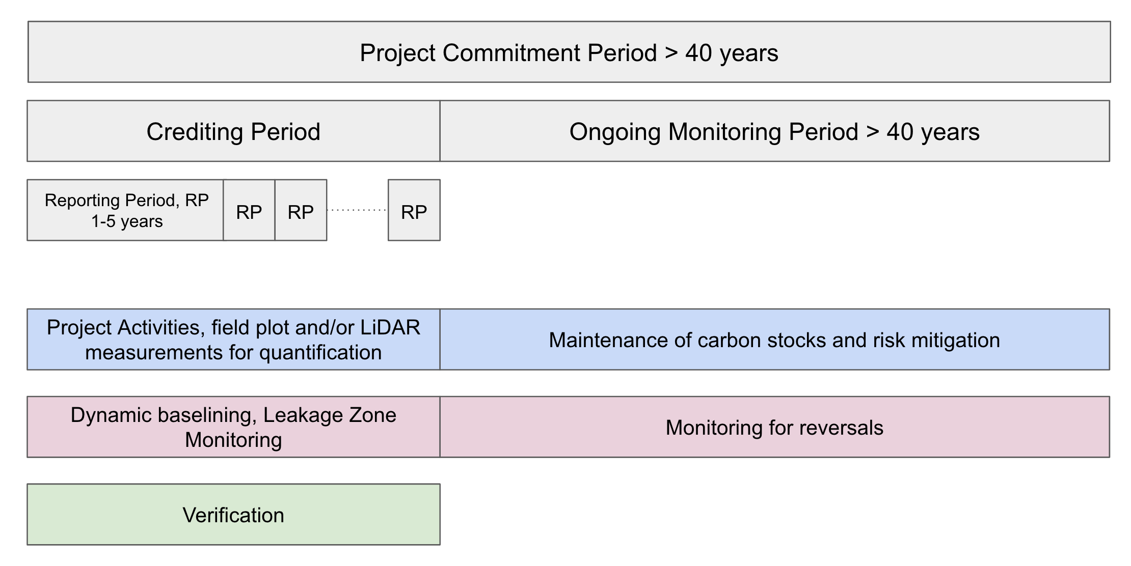
Figure 1 Summary of project periods. Colors represent actions owned by different stakeholders. Blue = Project Proponent. Green = VVB. Pink = Isometric.
5.6
Example Project Timeline
A project starting in 2025 has a Project Commitment Period of 100 years composed of a 40 year Crediting Period followed by 60 year Ongoing Monitoring Period. Credits issued have a 60+ year durability. Monitoring for quantification is conducted by the Project Proponent through the Crediting Period, and the reported activities are verified by a Validation and Verification Body (VVB) for each Reporting Period. At the end of the Crediting Period, maintenance of carbon stocks and monitoring for Reversals occurs for the remaining 60 years of the Project Commitment Period.
6.1
Overarching Principles
Following the Isometric Standard, Credits issued under this Protocol are contingent on the implementation, transparent reporting, and independent Verification of comprehensive safeguards. These safeguards encompass a wide range of considerations, including environmental protection, social equity, community engagement, and respect for cultural values. The process mandates that safeguard plans be incorporated into all major project phases, with detailed reports made accessible to stakeholders. Adherence to and verification of environmental and social safeguards is a condition for all Crediting Projects.
An environmental and social risk assessment in compliance with Section 3.7 of the Isometric Standard must be completed to identify potential risks, followed by the development of tailored mitigation plans. These plans must encompass specific actions to avoid, minimize or rectify identified impacts. Effective implementation of these measures must also be accompanied by a robust monitoring plan to detect adverse effects and pause project activities if necessary, using the principles of adaptive management described below.
Environmental and social risk identification, assessment, avoidance, and mitigation planning will be unique to the technical, environmental, and social contexts of The Project. To accommodate this variation, the requirements outlined in this section serve as a minimum to which the Project Proponent and Isometric can add risks on a case by case basis, to be included in the PDD, if applicable.
6.2
Governance and Legal Framework
Project Proponents must comply with all national and local laws, regulations and policies, and receive any necessary permits for project activities, if applicable. Where relevant, projects must comply with international conventions and standards governing human rights and uses of the environment.
Project Proponents must document activities that trigger environmental permitting requirements.
6.3
Adaptive Management
Adaptive management incorporates learnings and takeaways from project monitoring into project development12. Regular data collection and sharing is necessary to implement adaptive management. Results from data collection at the end of each Reporting Period must be shared with local stakeholders, as described in Section 6.5.1 of this Protocol, and be used to inform future iterations of project management and development.
Project Proponents are required to predict and plan for potential unintended outcomes of project activities and construct mitigation plans for such instances. Foreseeable risks identified during the preparation of the environmental and social risk assessment must be included in the PDD and the following must be detailed for each potential risk:
- A region specific mitigation plan
- The measured or observed outcome that will trigger the mitigation plan
- Plan for information sharing
- Emergency response plan, if applicable
The Project should not hinder the ability of the community or local ecosystem to adapt to climate change as a result of the CDR activity.
6.4
High Conservation Values
The High Conservation Values (HCV) Approach, developed by the HCV Network, identifies regionally specific facets of local communities and ecologies that must be considered during project developments resulting in land use change. The HCV Network has identified six values that may be at risk as a result of land use change projects. The values, along with corresponding requirements for Project Proponents to uphold them, are listed below:
- Species Diversity: Rare, threatened, endangered, or endemic species, at populations significant to regional, national, or global levels.
- Requirements. Population density of these species in the Project area must not decrease as a result of project activities (see Section 6.3.1). It is recommended that Project Proponents strive to increase the populations of these species during project activities to improve the climate adaptation potential of the local ecosystem, which in turn increases the durability of carbon stored in aboveground biomass.
- In cases where restoration will lead to a decrease in the population of rare, threatened, or endangered species which occupy non-forested or degraded lands, The Project may proceed if permitted by law and after a mitigation plan is developed in consultation with Isometric and included in the PDD. Mitigation plans must ensure no decrease in population density and should include activities such as:
- Translocation of populations to areas within the same region as the Project area, which can support and maintain the species' population;
- Maintenance of population in the Project area through the development of ecologically appropriate reserves and wildlife corridors;
- Active monitoring plans.
- In some instances, endemic species may be overpopulated prior to project initiation and decrease as a result of project activities. These or similar situations may be allowable under this Protocol, in consultation with Isometric. Project Proponents must demonstrate that a population decrease in the Project area will not adversely impact the species' metapopulation and that an endemic species was overpopulated in the Project area through one of the following:
- Peer-reviewed scientific literature;
- Authoritative national- or regional-body publications; or
- A population census conducted by an independent third party in consultation with Isometric.
- In cases where restoration will lead to a decrease in the population of rare, threatened, or endangered species which occupy non-forested or degraded lands, The Project may proceed if permitted by law and after a mitigation plan is developed in consultation with Isometric and included in the PDD. Mitigation plans must ensure no decrease in population density and should include activities such as:
- Requirements. Population density of these species in the Project area must not decrease as a result of project activities (see Section 6.3.1). It is recommended that Project Proponents strive to increase the populations of these species during project activities to improve the climate adaptation potential of the local ecosystem, which in turn increases the durability of carbon stored in aboveground biomass.
- Landscape-level ecosystems, ecosystem mosaics and intact forest landscapes: Broad-scale regions of interacting ecosystems which contain species in their natural patterns or distributions at populations significant on regional, national, or global scales.
- Requirements. Ecological integrity in the Project area must be maintained throughout project activities.
- Ecosystems and habitats: Rare, threatened, or endangered ecosystems or habitats.
- Requirements. Rare, threatened, and endangered ecosystems and habitats in the Project area must be maintained and protected throughout project activities.
- Ecosystem services: Fundamental ecosystem functions critical to ecological integrity and life, e.g., oxygen production, water filtration and protection of catchments, soil formation and erosion prevention, temperature regulation, nutrient cycling, habitat formation, provisioning of food and forage for fauna, etc.
- Requirements. Ecosystem services should be restored to those rendered by forests within the Project area region and maintained throughout project activities.
- Community needs: Commodities, resources, and community functions that are necessary for the livelihoods of local communities and Indigenous Peoples. This may include food, water, and infrastructure sources.
- Requirements. Community needs must be identified in consultation with local stakeholder groups. Community needs must not be damaged as a result of project activities. Access to community resources must not be limited as a result of project activities.
- Cultural values: Sites, landscapes, and habitats of significant cultural, historical, religious, economic, or archaeological value to local communities, Indigenous Peoples, or other groups identified to engage in those locations.
- Requirements. Cultural values must be identified in consultation with local stakeholder groups. Cultural values must not be damaged as a result of project activities.
For each value above, the Project Proponent must identify in the PDD if the value is present or absent in the Project area. This list must be constructed in consultation with relevant stakeholder groups, as identified in Section 6.5.1 and carried out in accordance with Section 3.5 of the Isometric Standard. The Stakeholder Engagement Plan for HCV identification must also be included in the PDD.
If a value is absent from the Project area, the Project Proponent must provide an explanation or justification such as survey results or recent publications. If a value is present in the Project area, the Project Proponent must include a plan to monitor and protect it throughout the Project Commitment Period in the PDD. We encourage Project Proponents to review the Common Guidance for the Management and Monitoring of HCV in developing this plan. If protection is not feasible during the Project activities and an HCV is damaged as a result of project activities, the Project Proponent must provide a restoration plan to return the area to its prior condition and quality.
If an HCV is threatened or damaged by forces or parties outside of the Project Proponent's jurisdiction and not as a result of or response to project activities, the Project Proponent must report such instances to Isometric, but may not be responsible for enacting a restoration plan. Failure to properly identify, monitor, and protect an HCV may result in the cessation of Credits.
6.4.1
Rare, Threatened, and Endangered Species
The Project Proponent must provide due diligence to ensure that the population density of rare, threatened, and endangered species in the Project area does not decrease, nor are new species added to this list, as a result of project activities. If either of these adverse impacts do occur, the Project Proponent must work with Isometric and the VVB to identify sources and explanations for these impacts in order to rule out project activities as the primary cause.
It is recommended that Project Proponents strive to increase the population of rare, threatened, and endangered species. Endangered species are defined as species under threat of extinction from all or a significant amount of their natural habitat. Threatened species are defined as those that are at risk of becoming endangered. Rare species are defined as those uncommon and found in isolated geographical locations. Project Proponents must consult local authorities for further regulations on these or similar groups. If local regulations exist, the Project Proponent must state them in the PDD.
The Project Proponent must consult reputable and current sources on rare, threatened, and endangered species to develop a list of these species, in the following order of priority:
- Local and/or regional registries;
- National registries;
- Peer-reviewed publications; and
- The International Union for Conservation of Nature (IUCN) Red List of Threatened Species15.
- For the purposes of this Protocol, the IUCN Red List designation of Vulnerable (VU) shall be considered Threatened, and Near Threatened (NT) shall be considered Rare.
The results of the rare, threatened, and endangered species list review must be included and referenced in the PDD.
For each rare, threatened, or endangered species identified, the Project Proponent must list the following in the PDD:
- Ecosystem services vital to the ecology and population stability of the rare, threatened, or endangered species found in the Project area.
- How The Project will maintain or enhance these ecosystem services so as to promote the survival of the rare, threatened, or endangered species.
- A population monitoring plan if there is an identified risk to the species as a result of Project activities. We encourage Project Proponents to consult Isometric, external subject matter experts, and/or authoritative resources in developing their plan.
The Project Proponent must handle data and information related to rare, threatened, and endangered species with discretion for the protection of these species, especially regarding species and/or regions that have histories of poaching, over-harvesting, or other elevated threats to population density and livelihoods.
6.5
Safeguarding of Biodiversity
As stated in Section 4.1, restoration projects must occur on degraded lands or lands that were historically classified as mangroves to be eligible for crediting under this Protocol. Because of this applicability requirement and the nature of restoration projects to plant and maintain species in the Project area, mangrove restoration projects are well placed to restore historic biodiversity in the region.
The species used for restoration must follow the principles outlined below.
6.5.1
Species Selection for Restoration
Mangrove species are taxonomically diverse, encompassing multiple families and several dozen genera. Species selected for restoration must be scientifically recognized as a mangrove species. Acceptable scientific sources include but are not limited to Duke et al. (1998)16 and Hogarth (2015)17. The species must be appropriate for both the geographic region and the Restoration Zone (see Section 4.2).
The Project Proponent must list the species planted and/or maintained in the Project area via project activities in the PDD.
In addition to mangrove species, Project Proponents may also plant other native species that naturally co-exist with mangroves but are not considered mangroves themselves, and would enhance the ecological integrity of the area. These species should not be the predominant species planted within the Project area. For the purposes of this Protocol, native species are defined as:
- Species indigenous to the Project area that would be found naturally (not planted or introduced anthropogenically via assisted migration) in the Project area prior to deforestation or degradation, and/or species that are indigenous to and found naturally in land adjacent to the Project area; or
- Species indigenous to the region that have not grown in the Project region for the past 100+ years due to displacement via anthropogenic factors or competition from invasive species, but are still well suited to the climate of the Project area, as demonstrated by scientific literature, presence of these species in similar climates, and/or evidence of displacement via one of these two forces.
- Indigenous species that have not existed in the Project region for the past 100+ years due to failure to adapt to changing climatic conditions may not be suitable for reintroduction for the purposes of GHG removal, but may be suitable for other ecosystem benefits. Reintroduction of such species should be done in consultation with Isometric.
Project Proponents must not introduce species invasive to the region or similar climates, geographies, or ecosystems of the Project area18, 19. The definition of 'invasive species' in this Protocol is consistent with the Convention on Biological Diversity's definition of Invasive Alien Species, being a "species whose introduction and/or spread threaten[s] biological diversity"20. Projects that plant invasive species will not be eligible for crediting under this Protocol. Additionally, Project Proponents must not introduce any species that harm rare, threatened, or endangered species or adversely impact the integrity of rare, threatened, or endangered ecosystems and habitats (see Section 6.3). Project Proponents are highly encouraged to consult with Isometric, the VVB, and/or external subject matter experts to ensure that species included in the restoration plan meet these requirements and the criteria described below.
6.6
Safeguarding of Community Livelihoods
6.6.1
Stakeholder Engagement
In accordance with Section 3.5 of the Isometric Standard, Project Proponents must demonstrate active stakeholder engagement throughout project planning and operation, ensuring that all risk mitigation strategies contribute to sustainable project outcomes. Local stakeholders may contribute an in-depth understanding of the Project area and operations, and provide invaluable insights and recommendations on potential risks, necessary safeguards and specific monitoring needs. Engaging local stakeholders in restoration projects creates community buy-in, providing long term commitment and investment in the success of restoration projects21, 22. Furthermore, lack of community support, stakeholder engagement, and perceived community benefits has been identified as a primary source of project failure in previous forestry projects23.
The Project Proponent must develop a Stakeholder Engagement Plan in accordance with the requirements outlined in Section 3.5 of the Isometric Standard. The plan and supporting documentation, including evidence of meetings or other forms of engagement, must be submitted in the PDD.
Prior to the commencement of project activities, Project Proponents are required to assess if Indigenous Peoples will be impacted by project activities. Impacts may include, but are not limited to:
- Project activities that occur on land or territories that are owned, occupied, or utilized by Indigenous Peoples, regardless of whether or not this claim is recognized by the local governing body or held by rights to self-determination, as recognized by the United Nations;
- Project activities that will affect natural resources necessary for the livelihoods or cultural rights of Indigenous Peoples.
Project Proponents must consult a reputable third party or subject matter expert to assess if Indigenous Peoples will be impacted by project activities. The results of this report must be included in the PDD. If the report identifies potential impacts to Indigenous Peoples, the Project Proponent must enact a Stakeholder Engagement Plan consistent with the principles of Free, Prior, and Informed Consent (FPIC) as outlined by the United Nations (UN) Declaration on the Rights of Indigenous Peoples24 in 2007 and expanded upon by the Food and Agriculture Organization of the United Nations in 201625.
- Free: Stakeholders are not subject to intimidation, coercion or manipulation during the decision making process.
- Prior: Engagement is sought in the early stages of project development before commencement of project activities. Consent must be sought as part of project development, regardless of local requirements. The timeline for the decision making and deliberation periods is set in consultation with all stakeholder groups and is informed by customary, local, and/or traditional practices.
- Informed: Information is presented in a manner that is accessible to all stakeholder groups. Accessible content may differ across stakeholder groups. The Project Proponent must consider in the information sharing process the language and medium of communication. For example, if information is presented electronically, stakeholders must have access to and familiarity with the necessary technology to review the information. If information is presented during in-person meetings, the meetings must be held at a time and in a location that is conducive to stakeholder attendance. Information presented to stakeholders must be objective and present trade-offs fairly and accurately. Finally, information must be provided on an ongoing basis. The following due diligence is strongly recommended to ensure stakeholder groups are well informed of project development and outcomes:
- Stakeholders should be made aware of the value of the Credits, and anticipated revenue of The Project at-large. The Project's anticipated growth and issuance should be modeled, and simulations describing the value of Credits at current market prices should be made clear to proponents.
- Stakeholders should have full access to the Project's finances, budget, and forecasted returns.
- Stakeholders should be aware of alternative land-use scenarios.
- Stakeholders should be aware of the value of the timber on The Project once the Crediting Period nears an end, so that they can better commit to conservation and upholding the contract.
- Stakeholders should have a clear understanding of the breakdowns in project income expenditure, and a clear understanding of the precise percentage of revenue that they are entitled to.
- Consent: Must be freely given and may be withdrawn. Consent may be conditional upon milestones in project development or the emergence of new information. Stakeholder consent is not guaranteed as a result of the Stakeholder Input Process.
The Project Proponent is encouraged to prepare alternatives for the withdrawal or denial of consent to project activities by stakeholder groups.
If required, the stakeholder engagement process must be enacted early in the Project development process, prior to the initiation of project activities. The stakeholder engagement schedule must be circulated prior to project initiation, and with enough notice to engage stakeholders in the planning processes. In some instances, Project Proponents that initiated project activities prior to engaging with Isometric and did not engage Indigenous Peoples stakeholders under the principles of FPIC may still be eligible for crediting under this Protocol, in consultation with Isometric, by demonstrating how stakeholder engagement will be incorporated into future project planning.
The following may serve as burdens of proof that the Stakeholder Input Process conforms with the principles of FPIC. The Project Proponent must indicate how these steps in the stakeholder engagement process were or will be carried out during the Project lifetime. Multiple rounds of stakeholder engagement may take place during a project lifetime, as needed. The Project Proponent may identify other burdens of proof demonstrating that the principles of FPIC have been observed and submit them in the PDD in addition to, or instead of, those below, in consultation with Isometric.
- Measures taken to effectively reach (i.e., identify and locate) all stakeholder groups. If the Project Proponent is not able to reach all adult community members, the percentage of adults in the community reached must be included in the PDD, as well as proof of the attempt to reach the remaining community members. The majority of adult community members must be successfully reached to be eligible for crediting under this Protocol.
- The manner in which information was presented to stakeholders, including the medium and language.
- How stakeholder input was obtained, including the medium and language.
- How stakeholder input was incorporated into the Project design.
The VVB may conduct random surveys or interviews with stakeholder groups, and/or witness some or all of the processes described above.
Project Proponents that do not identify Indigenous Peoples that will be affected by project activities are encouraged to consider if other relevant stakeholders rely on land or resources located within the Project area, and engage them following the principles of FPIC described above. All stakeholder groups and local communities have valuable and unique perspectives on developments in the Project area, which can contribute to project success.
The following information from the stakeholder engagement process must be made publicly available, with personal information anonymized or redacted to protect stakeholders, project personnel, and project outcomes. This may include:
- Due diligence that the FPIC processes were carried out (e.g., meeting recordings or copies of information shared with stakeholders)
- Budget reports, including revenue sharing agreements
6.6.2
Community Well-being and Impacts
6.6.2.1
Community Well-being
The Project Proponent must identify and develop processes for the protection and promotion of community well-being in the PDD, as follows:
- Protection of human rights:
- Policies and practices upholding anti-discrimination on the basis of gender, sexual orientation, etc.
- Grievances, feedback, and complaints:
- The process by which the Project Proponent accepts grievances, feedback, and complaints. Project Proponents must consult a third party to address grievances. The grievance redress process must be outlined in the PDD.
- Mediation and resolution process for grievances and complaints.
- Employment Opportunities:
- Hiring practices and policies, including the number of short-, medium-, and long-term employment opportunities that were recruited for in the local community relative to total new jobs created.
6.6.2.2
Community Impacts
As previously mentioned, community buy-in is critical to the success of a restoration project26, 27, 28. Community buy-in may be established when stakeholders are properly informed about the benefits they can expect from the restoration project. Equally important in maintaining buy-in is for the positive impacts resulting from the Project to match the (perception of) potential benefits presented to community stakeholders at the Project onset. A mismatch in benefits expected and benefits realized may similarly hinder project success.
While this Protocol will not prescribe requirements for community impacts, the Project Proponent is strongly encouraged to consider establishing the following programs and activities:
- Employment opportunity programs favoring local community members, especially in the creation of long-term jobs;
- Establishment of community benefit-sharing arrangements;
- Construction of infrastructure, such as roads, that are accessible to the community;
- Development of site specific mitigation plans for potential negative community impacts.
Positive impacts should be felt by all stakeholder groups identified in Section 6.5.1. Project Proponents should consider which groups may face the brunt of negative community impacts, and how positive community benefits may be shared equitably with these and other marginalized groups.
It is recommended that the Project Proponent provide support to the local communities and ecosystems to establish region specific mitigation strategies to adapt to changing climates.
7.0
Relation to Isometric Standard
The following topics are covered briefly in this Protocol due to their inclusion in the Isometric Standard, which governs all Isometric Protocols. See in-text references to the Isometric Standard for further guidance.
7.1
Project Design Document
For each specific Project to be evaluated under this Protocol, the Project Proponent must document project characteristics in a Project Design Document (PDD) as outlined in Section 3.2 of the Isometric Standard. The PDD will form the basis for project Validation and evaluation in accordance with this Protocol.
7.2
Verification and Validation
Projects must be validated and net CO2e removals verified by an independent third party, consistent with the requirements described in this Protocol, as well as in Section 4 of the Isometric Standard.
The Validation and Verification Body (VVB) must consider the following requisite components:
- Verify that The Project meets the Applicability conditions described in Section 4
- Verify that the Environmental & Social Safeguards outlined in Section 6 are met
- Verify that the System Boundary & Leakage assessment adheres to the requirements of Section 8
- Verify that the quantification approach and monitoring plan adheres to requirements of Section 9
- Verify that the conditions for ensuring durability and monitoring for Reversals in Section 10 are met
- Verify that The Project is compliant with requirements outlined in the Isometric Standard
As part of this evaluation, the VVB must also review the characterization and quantification of all individual uncertainty sources within the listed components that contribute to the calculation of net CO2e removal.
7.2.1
Verification Materiality
The threshold for Materiality, considering the totality of all omissions, errors and misstatements, is 5%, in accordance with Section 4.3 of the Isometric Standard.
Verifiers should also verify the documentation of uncertainty of the GHG Statement as required by Section 2.5.7 of the Isometric Standard. Qualitative Materiality issues may also be identified and documented, such as:
- Control issues that erode the verifier's confidence in the reported data;
- Poor management documented information;
- Difficulty in locating requested information; and
- Noncompliance with regulations indirectly related to GHG emissions, removals or storage
7.2.2
Site Visits
Project Validation and Verification must incorporate site visits to project facilities, namely in situ field plots, in accordance with the requirements of ISO 14064-3, 6.1.4.2. This is to include, at a minimum, site visits to the Project site during Validation and initial Verification. Validators should, whenever possible, observe project operations to ensure full documentation of process inputs and outputs through visual observation (see Section 4 of the Isometric Standard).
Additional site visits may be required if there are substantial changes to field operations over the course of Validation, or if deemed necessary by Isometric or the VVB. Site visit plans are to be determined according to the VVB's internal assessment, in consultation with Isometric.
7.2.3
Verifier Qualifications and Requirements
Verifiers and Validators must comply with the requirements defined in Section 4 of the Isometric Standard. In addition, verification teams must maintain and demonstrate expertise associated with the specific technologies of wetland restoration including both field measurements and Earth System remote sensing data processing and analysis.
7.3
Ownership
CDR via mangrove restoration is a result of a multi-step process (e.g., propagule planting, managing hydrological conditions, monitoring), with activities in each step potentially managed by a different operator, company, or owner. A single Project Proponent must be specified contractually as the sole owner of the Credits when there are multiple parties involved in the process, and to avoid Double Counting of net CO2e removals. Contracts must comply with all requirements defined in Section 3.1 of the Isometric Standard.
7.4
Additionality
The Project Proponent must be able to demonstrate additionality through compliance with Section 2.5.3 of the Isometric Standard. The Baseline scenario and Counterfactual utilized to assess additionality must be project-specific and comply with Section 9.4 of this Protocol.
Government subsidies or civil contractual obligations for restoration, such as organization bylaws, inhibit additionality and fall under the Regulatory criteria in Section 2.5.3 of the Isometric Standard. Additionality is assessed each Reporting Period using dynamic baselining as outlined in Section 9.4.
Additionality determinations should be reviewed and completed at every Verification at a minimum, or whenever project operating conditions change significantly, such as the following:
- Regulatory requirements or other legal obligations for project implementation change or new requirements are implemented;
- Project financials indicate Carbon Finance is no longer required to operate the Project.
If a review indicates the Project has become non-additional, the Project will be ineligible for future Credits. Current or past Crediting Periods will not be affected.
7.4.1
Common Practice
The following steps must be taken to demonstrate that without Carbon Finance the Project activity is not Common Practice, in accordance with the requirements defined in Section 2.5.3.1 Common Practice Analysis of the Isometric Standard.
- Define the Project activity (e.g., propagule planting).
- Identify the applicable geographic area, as described in Section 2.5.3.1 Common Practice Analysis of the Isometric Standard.
- Identify a similar class of adopters or landowners (e.g., aquaculture, community-held land, private concessions).
- Identify and explain any essential distinctions between the proposed Project and similar activities, as described in Section 2.5.3.1 Common Practice Analysis of the Isometric Standard.
- Assess the market penetration rate using either a) a survey-based approach, or b) using relevant data from existing literature, as follows:
- a) Survey-based approach:
- Survey a representative sample of similar landowners from within the relevant geographic domain within five years of the Project start date.
- Calculate the cumulative market penetration rate (as a percentage) of the Project activity by landowners who have not received Carbon Finance revenue (e.g., are neither part of a registered Isometric Project, nor registered under other GHG programs) in the sample of adopters.
- b) Data from existing literature: Statistics on restoration activities derived from data collected within five years of the Project start date may be used for this demonstration, provided they are relevant to the Project area, do not distinguish between activities incentivized by and not incentivized by Carbon Finance (thus are conservative), and are publicly available as:
- i) agricultural or aquacultural census, survey or other government data;
- ii) peer-reviewed scientific literature; or
- iii) independent research or reports, with full and transparent methods and documentation of results.
In accordance with Section 2.5.3.1 Common Practice Analysis of the Isometric Standard, the proposed Project activity is considered to demonstrate Common Practice additionality where the market penetration rate is below or equal to 20%.
7.5
Uncertainty
The uncertainty in the overall estimate of the net CO2e removal as a result of The Project must be accounted for. The total net CO2e removed for a specific Reporting Period, , , must be conservatively determined in accordance with the requirements outlined in Section 2.5.7 of the Isometric Standard.
7.5.1
Reporting of Uncertainty
Projects must report a list of all key variables used in the net CO2e removal calculation and their individual uncertainties, as well as a description of the uncertainty analysis approach, including:
- field measurements used for the net CO2e removal calculation
- parameters that impact the estimation of the total aboveground woody biomass, such as allometric equation parameters, canopy height, wood density, etc.
- parameters used for calculating carbon stocks, including root-to-shoot ratios and carbon fractions
- parameters used for soil organic carbon estimation, including estimates of organogenic vs minerogenic components
- emission factors utilized, as published in public and other databases used
The uncertainty information should at least include the minimum and maximum values of each individual variable. More detailed uncertainty information should be provided if available, as outlined in Section 2.5.7 of the Isometric Standard.
In addition, a sensitivity analysis that demonstrates the impact of each input parameter uncertainty on the final net CO2e uncertainty must be provided. Details of the sensitivity analysis method must be provided such that a third party can reproduce the results. Input variables may be omitted from an uncertainty analysis if they contribute to a < 1% change in the net CO2e removal. For all other parameters, information about uncertainty must be specified.
7.6
Data Sharing
In accordance with the Isometric Standard, all evidence and data related to the underlying quantification of CO2e removal and environmental and social safeguards monitoring will be available to the public through the Isometric platform. That includes:
- Project Design Document
- See Section 11 for a list of pre-deployment requirements that must be included in the PDD
- GHG Statement
- Measurements taken, with supporting documentation (e.g., calibration certificates)
- Emission factors used
- Scientific literature used
- Proof of approval for necessary permits
- Remote sensing and field plot data collected by The Project
- All maps generated for calculating carbon stocks in the Project area
- All maps generated for calculating carbon stocks in control areas (geospatial reference data can be removed for privacy reasons)
- All data and methodological details used for the baseline calculation
- Model specifications and output
The Project Proponent can request certain information to be restricted (only available to authorized Buyers, the Registry, and VVB) where it is subject to confidentiality. This includes emission factors, specific data, and/or proprietary models from licensed databases. However, all other numerical data produced or used as part of the quantification of net CO2e removal will be made available.
8.0
System Boundary, Project Baseline, and Leakage
8.1
System Boundary
The scope of this Protocol includes the GHG sources, sinks, and reservoirs (SSR) associated with a mangrove restoration project.
A cradle-to-grave GHG Statement must be prepared encompassing the GHG emissions relating to the activities outlined within the system boundary.
GHG emissions and removals associated with The Project may be direct emissions from a process, or indirect emissions from combustion of fuels, electricity generation, or other sources. Emissions must include all GHG SSRs within the system boundary, from the construction or manufacturing of each physical site and associated equipment, closure and disposal of each site and associated equipment, and operation of each process, including embodied emissions of equipment and consumables used in the Project. The Project Proponent is responsible for identifying all sources of emissions directly or indirectly related to project activities.
Any emissions from sub-processes or process changes that would not have taken place without the CDR Project must be fully considered in the system boundary. Any activity that ultimately leads to the issuance of Credits should be included in the system boundary.
The system boundary must include all relevant GHG SSRs controlled, related and affected by The Project, including but not limited to the SSRs set out in Table 1. If any GHG SSRs within Table 1 are deemed not appropriate to include in the system boundary, they may be excluded provided that robust justification and appropriate evidence is provided in the PDD.
Table 1. Scope of activities and GHG SSRs to be included in the system boundary.
| Activity | GHG source, sink or reservoir | GHG | Scope | Timescale of emissions and accounting allocation |
|---|---|---|---|---|
| Project establishment | Equipment and materials | All GHGs | Embodied emissions associated with equipment and materials manufacture related to project establishment (lifecycle modules A1-329). This must include product manufacture emissions for: • Equipment (e.g., vehicles or machinery) • Buildings/structures (e.g., on-site nurseries) • Infrastructure (e.g., roads or footpaths) • Temporary structures (e.g., tree shelters, fencing) | Before project operations start - must be accounted for in the first Reporting Period or amortized in line with allocation rules (See Section 9.5.1) |
| Equipment and materials transport to site | All GHGs | Transport emissions associated with transporting materials, equipment and seedlings to the Project site(s) (lifecycle module A4). | ||
| Planting and installation | All GHGs | Emissions related to construction and installation of the Project site(s) (lifecycle module A5). This must include, as appropriate: • Energy use for planting, installation and groundworks • Waste processing activities • Land use change, including emissions associated with dredging (see Section 9.5.1.1) • Site clearance, including biomass burning • Emissions associated with changing salinity and nitrate inputs inside and outside of the Project area | ||
| Misc. | All GHGs | Any SSRs not captured by categories above (e.g., staff travel). | ||
| Operations | Mangroves management | All GHGs | Emissions related to mangrove forest management activities (e.g., pruning, weeding, pest control, biomass burning and watering). This must include embodied emissions of equipment, as well as consumables such as water, fertilizers and pesticides. | Over each Reporting Period - must be accounted for in the relevant Reporting Period (see Section 9.5.2). |
| Maintenance | All GHGs | Maintenance of the project area, including any repair or replacement of equipment, vehicles, buildings and infrastructure. | ||
| Monitoring, Reporting and Verification (MRV) | All GHGs | Emissions related to MRV activities (e.g., measurements, sampling, or commissioning LiDAR flights). | ||
| CO₂ stored | CO₂ | The gross amount of CO₂ removed and durably stored in living biomass, and organogenic soils (see Section 9.3). | ||
| Misc. | All GHGs | Any SSRs not captured by categories above (e.g., staff travel). | ||
| End-of-Life | Ongoing monitoring | All GHGs | Emissions relating to monitoring activities over the Project Commitment Period. | After Reporting Period - must be estimated and accounted for in the first Reporting Period or amortized in line with allocation rules (see Section 9.5.3) |
| Ongoing mangrove management | All GHGs | Emissions relating to ongoing project management activities over the Project Commitment Period. | ||
| Misc. | All GHGs | Any SSRs not captured by categories above (e.g., ongoing staff travel). |
Miscellaneous GHG emissions are those that cannot be categorized by the GHG SSR categories provided in Table 1. The Project Proponent is responsible for identifying all sources of emissions directly or indirectly related to project activities and must report any outside of the SSR categories identified as miscellaneous emissions.
Emissions associated with The Project's impact on activities that fall outside of the system boundary of The Project must also be considered. This is covered under Leakage in Section 8.3.
In line with the GHG Accounting Module v1.0, the Project must:
- Consider all GHGs associated with SSRs, in alignment with the United States Environmental Protection Agency’s definition of GHGs. This includes: carbon dioxide (CO2), methane (CH4), nitrous oxide (N2O) and fluorinated gasses such as hydrofluorocarbons (HFCs), perfluorocarbons (PFCs), sulfur hexafluoride (SF6) and nitrogen trifluoride (NF3). For CO2 stored, only CO2 will be included as part of the quantification. For all other activities, all GHGs must be considered. For example, the release of CO2, CH4, and N2O is expected during diesel combustion;
- Quantify emissions in tonnes CO₂ equivalent (t CO₂e) using the 100-year Global Warming Potential (GWP) for the GHG of interest, based on the most recent volume of the IPCC Assessment Report (currently the Sixth Assessment Report); and
- Consider Materiality of SSRs in line with Isometric requirements. Project Proponents may exclude SSRs where the total emissions for that SSR, and all excluded SSRs collectively, are expected to be < 1% of net CO2e removals.
See Section 2.4.2.1 of the GHG Accounting Module
8.2
Project Baseline
The Baseline scenario for restoration assumes that the activities associated with The Project do not take place and that any infrastructure associated with The Project is not built.
The Counterfactual is the CO2 stored that would have occurred due to natural regeneration of biomass over the Crediting Period in the absence of The Project. This Protocol uses a dynamic baseline approach to quantify the Counterfactual. This is detailed in Section 9.4.4.
8.3
Leakage
8.3.1
Overview of Leakage Assessment
Leakage emissions, , occur when project activities lead to emissions that occur outside the system boundary of restoration projects. They include increases in GHG emissions as a result of restoration projects displacing emissions or causing a secondary effect that increases emissions elsewhere. Three key types of leakage can occur for restoration projects:
- Activity-shifting leakage. Mangrove restoration projects may displace activities in their Project areas, leading to an increase in those activities outside of the Project area, which may result in potential land conversion. Examples are where the local community can no longer use the Project site for subsistence, or where farming is displaced as a result of project activities. This type of leakage is known as "Direct" leakage as the relevant stakeholders can be identified and the activity-shifting is traceable.
- Market leakage. Mangrove restoration projects may displace activities, which results in a reduction in supply of a commodity. Changes to the supply and demand equilibrium causes other market actors to shift their activities, leading to potential land conversion. This type of leakage is known as "Indirect" leakage because its effects cannot be isolated and measured directly. Quantifying the likelihood and potential magnitude of market leakage is complex and relies heavily on modeling and available literature.
- Ecological leakage. Project activities may lead to an increase in emissions in areas outside of the Project site as a result of ecological interactions, for example changing hydrological conditions that lead to increased methane(CH4) or nitrous oxide (N2O) emissions. Project activities that adversely alter the water table, harming ecological integrity within the Project area and surrounding landscape and watershed, are not permitted under this Protocol. Isometric will review all proposed hydrological modifications laid out in the PDD (see Section 4.1.1). If any activities are deemed to be a significant risk to increasing GHG emissions (i.e., CH4 and N2O), the Project will be ineligible. Therefore, projects that are eligible under this Protocol will have a low risk of ecological leakage.
The overall process for addressing activity-shifting and market leakage is set out in the flowchart in Figure 2.

Figure 2. Flowchart of process for addressing activity-shifting and market leakage.
The flowchart is based on the following principles:
- If the commodity was used for subsistence this presents a risk of activity-shifting leakage.
- Activity-shifting leakage risk can be directly identified and mitigated.
- If the commodity was commercial, there is always a risk of market leakage.
- If the commodity was commercial, there might also be a risk of activity-shifting leakage.
- Where Direct Actors have been identified as impacted, activity-shifting leakage mitigation activities will address both activity-shifting leakage and market leakage. However, if only market leakage mitigation is implemented, this will not satisfy the activity-shifting leakage risk. For this reason, if only market leakage mitigation is undertaken, additional activity-shifting leakage monitoring must take place. If only partial or no leakage mitigation is in place, then the market leakage deduction must be applied, as well as a requirement for activity-shifting leakage monitoring.
- Where the commodity was used for subsistence and is not mitigated in full, The Project is not eligible. This is on the grounds of a very high risk of activity-shifting leakage due to dependencies on the land, but also because the Project area was an area fundamental for the livelihoods of communities.
- Leakage mitigation has different requirements depending on whether it is addressing activity-shifting leakage or market leakage.
8.3.2
Pre-Project Information
Implementation of the flowchart for addressing activity-shifting and market leakage (Figure 2) requires an understanding of Pre-Project Productivity, , including pre-project information about Direct Actors and how the commodity was used. Direct Actors are defined as site owners, tenants or other users that engaged with the Project site in a way that produced commodities before the Project activities commenced.
The information required is set out below:
- including the type of commodity and yield; and
- Whether the commodity was used for subsistence or commercial production.
- For the purposes of this assessment, commodities that are commercial, but primarily sold to the local community, are considered subsistence.
8.3.2.1
Determining Pre-Project Productivity, PPP
is defined as the annual productivity of a commodity type at the Project site in relevant units (e.g., tonnes/ yr). This should be an average of the three years of production prior to the Project activities starting.
The data hierarchy for obtaining information for is set out below:
- Farm or aquaculture records or permits, including physical production records and financial logs including income and expense records and receipts;
- Land registry data which details previous land holdings at the Project site and production information related to land holdings; or
- Remote sensing data which can be used to inform commodity production, with support from municipal data and scientific literature values, as available.
The hierarchy must be followed and data choices evidenced. For example, if land registry data is used, sufficient evidence of no available farm records will be required. Sufficient evidence may include, but is not limited to, official government statements, reports, or affidavits and/or written sworn statements or affidavits by Direct Actors regarding the lack of records.
As part of determination of , the Project Proponent must confirm the following:
- The type of commodity, , that existed at the Project site pre-project (see Section 8.3.3.1.1)
- The productivity of commodity production, (see Section 8.3.3.1.1)
8.3.2.1.1
Type of Commodity, c
The following considerations and assumptions should be made when determining the type of commodity, :
- Where land registry data is used to determine commodity type and commodities produced by one land holding are not quantified separately, or spatially separated, the most conservative assumption on commodity type for the site as a whole must be made. The most conservative assumption should be determined by running the calculations for (see Equation 5) assuming 100% of the production for each commodity and zero mitigation. The commodity that contributes to the highest value for should be assumed as full commodity production at the site.
- Where remote sensing data is used:
- Conservative assumptions on commodity type must be made in any areas of uncertainty. Any assumptions made must be transparently documented and justified.
- If the land use changed within the five years prior to the Project start date, for example from charcoal production to aquaculture, the most recent commodity type should be used if it was in use for at least one year.
- If more than one commodity type is identified, they must both be assessed as part of the leakage assessment provided that the spatial extent of each commodity type is clear.
8.3.2.1.2
Productivity of Commodity Production, Yc
Productivity must be reflective of an average of the three years prior to the Project activities starting.
The following considerations and assumptions should be made when determining productivity:
- Farm records must reflect the most recent relevant commodity or ownership class where estimates have been disaggregated by those attributes, and must be substantiated with a signed attestation from the farmer or landowner.
- Any assumptions made to interpret productivity data from farm records or land registry data must be of a conservative nature and be transparently reported.
- Methodologies that determine productivity data from remote sensing may be reviewed on a case by case basis. Models must be regionally- and commodity-appropriate and should have a minimum observation frequency of twice per year over a three-year period. Any inferences of productivity made using remote sensing data must be clearly referenced and justified. These must be of a conservative nature and be transparently reported. Future revisions of this Protocol will consider appropriate requirements for using remote sensing data to determine productivity as standard methodology.
- Where productivity related information is not available, average yield for the region may be used as a proxy for productivity. An average over the last five years must be taken to account for anomalies.
- Where region-specific data is not available, average yield data at a national level may be used as a proxy for yield. For example, annual yield data for the commodity type from the Food and Agriculture Organization of the United Nations. An average over the last five years must be taken to account for anomalies.
- Where regional or national averages are not available for fuelwood production, average above-ground biomass growth rates published by the IPCC that are applicable to the region should be used.
8.3.2.2
How the Commodity was Used
The Project Proponent must determine the previous use of the commodity and whether it was:
- A commercial commodity: a commodity that is destined for regional, national, or global commercial markets; or
- A subsistence commodity: a commodity that is not destined for regional, national, or global commercial markets and is consumed by the local community.
The Project Proponent must determine this using the following information:
- An affidavit from the identified Direct Actors confirming the end-users of the commodity, or the majority buyer(s) the commodity was sold to. Direct Actors must include the previous site owners, tenants, or other users that engaged with the Project site in a way that produced commodities.
- An affidavit from the local authority claiming that the Project area was publicly owned and used for subsistence.
- An affidavit from members of the local community confirming that the Project area was used for subsistence.
- An affidavit or records from local intermediaries such as wholesalers, distributors, food processors, grain elevators, or livestock auctions, confirming that they purchased commodities from the Project site in the past.
If it is not possible to determine whether the commodity was for subsistence or commercial use, then the Project Proponent must assume it was subsistence.
8.3.2.3
Evidencing Zero Pre-Project Productivity
If the Project determines that is zero, this must be evidenced appropriately. This includes:
- Evidence of no farm records on open source sites;
- Land registry data which details no previous agricultural land holdings at the Project site;
- Self-assessment from Direct Actors regarding prior use of the site, including photo evidence;
- Written confirmation from project site neighbors or community members regarding the prior use of the site, including photo evidence. This may be land owners or managers from adjacent areas. Where possible this must include a diverse range of stakeholders.
Evidence must be provided for three years preceding the Project Proponent's purchase of the site for restoration, or the Project start date, whichever is earlier.
In addition, Isometric will undertake remote sensing analysis on project sites which claim that is zero. Remote sensing mapping will be transparently displayed on the registry. Only where remote sensing analysis indicates there are no signs of agricultural or aquacultural production will the Project be eligible for claiming zero .
8.3.2.4
Calculation of CO2eLeakage
is part of the calculation of , as set out in Section 9.5.
is quantified with the following equation:
(Equation 1)
Where:
- is the total emissions associated with leakage during the first Reporting Period, , in tonnes CO2e.
- is the total emissions associated with market leakage for a Reporting Period, , in tonnes of CO2e, see Section 8.3.5.
- is the adjustment to leakage emissions as a result of activity-shifting leakage being identified via monitoring for a Reporting Period, , in tonnes of CO2, see Section 8.3.6.2.
- is total emissions associated with leakage mitigation activities for a Reporting Period, , in tonnes of CO2e, see Section 8.3.4.
is quantified for every Reporting Period, , however the following should be noted:
- is only estimated once during the first Reporting Period. The emissions associated with market leakage must be allocated to the first Reporting Period.
- is based on ongoing monitoring and therefore must be reported at every Verification. It is not reported during the first Reporting Period. For the first Reporting Period, and any preceding Reporting Periods where no activity-shifting leakage is identified, is zero. Activity-shifting leakage adjustments identified (up to a maximum of total possible leakage) should be allocated to the Reporting Period in which they are identified.
- must be allocated to the Reporting Period in which they occur. For example, emissions that occur as a result of establishment should be allocated to the first Reporting Period. Ongoing emissions, such as fuel use must be allocated to the Reporting Period in which they occur.
8.3.3
Leakage Mitigation
The aim of leakage mitigation activities is to reduce the amount of leakage by increasing production of the displaced commodity elsewhere. Leakage mitigation must take place in areas called Leakage Mitigation Sites. These must be separate to the Project site, but may be directly adjacent. Leakage mitigation activities should be equal to or greater than the expected displacement of production. The efficacy of mitigation will be assessed and appropriate deductions applied in the event that mitigation activities do not match the level of displacement (see Equation 2).
The following equation is used to calculate the effectiveness of leakage mitigation:
(Equation 2)
Where:
- is unmitigated Pre-Project Productivity of commodity, , in appropriate units (e.g., tonnes per year).
- is Pre-Project Productivity - average annual production of commodity that would have been produced in the absence of The Project, in appropriate units (e.g., tonnes per year).
- is Mitigation area productivity, in appropriate units (e.g., tonnes per year).
When is 0, the Project had zero productivity.
When is > 0 and is 0, the Project has achieved full leakage mitigation and does not take a market leakage emissions deduction.
When is > 0 and is > 0, the Project takes a market leakage emissions deduction.
Leakage mitigation requirements are different depending on whether mitigation is to address activity-shifting leakage (see Section 8.3.3.1) or market leakage (see Section 8.3.3.2). Activity-shifting leakage will also by nature address market leakage, however market leakage alone will not address activity-shifting leakage.
In addition to the leakage type specific requirements, all leakage mitigation activities must meet the following requirements:
- A written agreement must be in place stating that the landowner of the Leakage Mitigation Site allows the Project Proponent to uniquely claim the increases in productivity as leakage mitigation associated with the Project. This must be covered via legal agreements for a five year term.
- Leakage mitigation activities must provide support to landowners of the Leakage Mitigation Site for a minimum of five years. This is on the basis that the initial leakage mitigation activity leads to sustainable recurring revenue for landowners of the Leakage Mitigation Site.
- Leakage mitigation may lead to increased productivity via creating new production on lands that were not previously used for production, or via intensifying production on existing production lands.
- Land selected for leakage mitigation must not have any other productivity that is negatively impacted by mitigation.
- The mitigation activity must lead to an increase in productivity as a direct result of intentional action from the Project Proponent.
- The spatial extent of the Leakage Mitigation Site and full details of activity must be provided as part of the PDD.
8.3.3.1
Activity-Shifting Leakage Mitigation
For mitigation of activity-shifting leakage, the Project Proponent must have a full understanding of the information set out in Section 8.3.2.1. The mitigation must be informed by the Direct Actors and be undertaken in agreement with Direct Actors. Mitigation activities must lead to new productivity or productivity increases that directly benefit the Direct Actors. This likely means that the increase in production should be limited to the same commodity type, but this decision should be informed by the Direct Actors. This also likely means that the Leakage Mitigation Site should be in the same locality, but again this should be informed by the Direct Actors.
The Project Proponent should engage with Direct Actors associated with the site's prior productivity to understand how the Project activity impacted the previous users of the Project site. Direct Actors include the previous site owners, tenants or other users that engaged with the Project site in a way that produced commodities.
The Project Proponent must receive an affidavit from the identified Direct Actors confirming the following:
- Their occupation;
- How they previously used or engaged with the Project site;
- How the Project activities impacted their use of the Project site; and
- How they designed mitigation activities with the Project Proponent.
Full records of correspondence, including meeting notes, and signed agreements must be made available as part of the PDD.
If information from Direct Actors is unavailable, the Project Proponent will be unable to undertake activity-shifting leakage mitigation.
8.3.3.2
Market Leakage Mitigation
For mitigation of market leakage, the following must be true in addition to the requirements set out in Section 8.3.3:
- The mitigation may increase productivity of a similar substitute commodity, as this will result in a land sparing effect.
- The Leakage Mitigation Site should be in the same region. If this is not possible, the Leakage Mitigation Site must be in the same national boundary.
8.3.4
Calculating the Emissions Impact of Leakage Mitigation Activities,
The emissions impact of leakage mitigation activities, must be considered. The same system boundaries set out in Table 1 must be considered, noting that it is likely only certain GHG SSRs will be included. At minimum, the following emissions sources must be considered:
- Embodied Emissions associated with any new construction or materials (e.g., fencing);
- Emissions associated with fertilizer use (e.g., if fertilizers are used to increase productivity);
- Emissions associated with farm or aquaculture operations (e.g., fuel use and waste management); and
- Emissions associated with land clearance, including dredging activities, for mitigation activities.
Only activities that are additional as a result of the leakage mitigation activity should be considered as part of . Activities that were already occurring and would continue to occur without the leakage mitigation activity may be omitted from the emissions accounting, if evidence that the activity was already occurring and would have continued to occur in the absence of the leakage mitigation activity is provided.
8.3.5
Calculating Market Leakage Emissions, CO2eMarketLeakage
considers emissions associated with land conversion as a result of market leakage. It is noted that other emissions may result from market leakage, such as fertilizer use as part of intensification to produce an increase in commodity supply. These emissions sources have been excluded at this time given a lack of globally appropriate data availability. These emissions are also expected to be negligible compared to land conversion emissions.
If includes multiple commodity types, must be quantified for each commodity type.
Market leakage emissions are quantified using the following equations:
(Equation 3)
Where:
- is total leakage emissions, in tonnes CO2e.
- is the commodity type.
and:
(Equation 4)
Where:
- is induced land conversion to bring new land into production, in hectares.
- is the carbon stock factor for mangrove habitat, including biomass and soil organic carbon, in tonnes CO2 per hectare.
- is the commodity type.
8.3.5.1
Estimating Induced Land Conversion, haLC
Project Proponents are required to estimate the amount of new land brought into production, . This estimate must be informed by:
- Pre-Project Productivity of a commodity type at the Project site;
- the estimated proportion of this productivity that would be replaced with new production via an increase in supply of the commodity type;
- the increase in supply that would result in new land being brought into production; and
- the yield of new land being brought into production.
The new land brought into production must be calculated separately for each commodity type being displaced as a result of the Project.
Land conversion for production is quantified using the following equation:
(Equation 5)
Where:
- is induced land conversion to bring new land into production, in hectares.
- is adjusted unmitigated Pre-Project Productivity, in appropriate units (e.g., tonnes per year.)
- is increased Supply - proportion of foregone that will be replaced by increased supply elsewhere, as a percentage.
- is increased supply that will result in new land brought into production, as a percentage.
- is yield on new land brought into production, in appropriate production units (e.g., tonnes per hectare).
- is the commodity type.
8.3.5.1.1
Adjusted Unmitigated Pre-Project Productivity,
Adjusted unmitigated Pre-Project Productivity, , must be calculated using the following equation:
(Equation 6)
Where:
- is the adjusted unmitigated Pre-Project Productivity, in appropriate units (e.g., tonnes per year).
- is the unmitigated Pre-Project Productivity, average annual production of commodity that would have been produced in the absence of the Project, in appropriate units (e.g., tonnes per year).
- is the annual growth rate in productivity of the commodity type.
- is the commodity type.
8.3.5.1.2
Growth Rate, GR
The annual growth rate in productivity of the commodity type and region must be assigned as part of Equation 6. This is a requirement to ensure that any likely future increases in productivity are accounted for as part of the assessment.
Growth rate must be calculated based on the following hierarchy:
- Regional commodity specific data should be used to source yield values to determine growth rates, where available. For example from the United States Department for Agriculture for the commodity type and state;
- National commodity specific data for agriculture from FAOSTAT may be used to source yield values to determine growth rates.
Growth rate must be calculated using the following equation:
(Equation 7)
Where:
- is the growth rate, as a percentage.
- is the yield as sourced from regional or national datasets, in production unit per hectare per year.
- is the commodity type.
- is the most recent year of recorded yield data.
- is the historic year yield data.
Average growth rate is determined by taking the difference between yield in the most recent year of recorded data () and a historic year (). Where possible should represent 25 years prior to t. Where this is not possible, a minimum of 10 years prior to t is allowable.
If a recent negative shock leads to a negative growth estimate of yield growth, a value of zero should be used.
8.3.5.1.3
Estimating Increased Supply, IS
Increased Supply is the proportion of foregone productivity that will be replaced by increased supply elsewhere. This is underpinned by the premise that foregone production will not necessarily be replaced in totality by increased supply elsewhere as a result of elasticities of supply and demand. Global markets for commodities have been assumed for the purposes of the leakage assessment.
Estimates for are determined using the following equation:
(Equation 8)
Where:
- is increased supply, as a percentage.
- is elasticity in supply, as a ratio.
- is elasticity in demand, as a ratio.
- is the commodity type.
Guidance for estimating IS for a commodity can be found in Appendix A. Future version of this Protocol will provide default values for common commodities.
8.3.5.1.4
Estimating Increased Supply that will Result in New Land, NL, Being Brought into Production
considers the percentage of increased supply that will result in new land brought into production for the commodity type. This is underpinned by the premise that not all increased supply will result in new lands being brought into production. Some increased supply may be made up of intensification of activities and increased yields on existing production lands.
Guidance for estimating for a commodity can be found in Appendix A. Future version of this Protocol will provide default values for common commodities.
8.3.5.1.5
Estimating Yield on New Land, YNL, Brought into Production
, considers the yield on new land brought into production for commodity . To determine yield on new land, follow the regional and national approach set out in the assessment of Productivity (Section 8.3.2.1.1).
8.3.5.2
Determining the Carbon Stock Emission Factor, EFCarbonStock
must be derived from the IPCC average national aboveground biomass, belowground biomass and soil carbon content of mangroves. Mean carbon stocks should be derived from the following tables in the 2013 Supplement to the 2006 IPCC Guidelines for National Greenhouse Gas Inventories - Wetlands30:
- Aboveground biomass in mangroves estimates in Table 4.3;
- Ratio of belowground to aboveground biomass in mangroves in Table 4.5;
- Soil carbon stocks for mangroves in Table 4.11.
Carbon stocks should be determined using the same ratio of mass of CO2 to mass of , and carbon fraction, , as set out in Section 9.3.1.1.
8.3.6
Activity-Shifting Leakage Monitoring
Where activity-shifting mitigation is in place, activity-shifting leakage monitoring is not required. Where only market leakage mitigation is in place, activity-shifting leakage monitoring must be undertaken for the Project. This is because market leakage mitigation does not necessarily mitigate activity-shifting leakage and Direct Actors may still be implicated. Where only partial or no leakage mitigation is in place, activity-shifting leakage monitoring must be undertaken in addition to a full or partial market leakage emissions deduction.
Activity-shifting leakage monitoring requires satellite imagery of a buffer or boundary zone along the Project perimeter, called the Leakage Monitoring Zone. The Leakage Monitoring Zone will form a consistent buffer zone along the perimeter of the Project site. The distance between the exterior perimeters of the Project site and Leakage Monitoring Zone (i.e., the buffer width) will be determined by the smaller of the following:
- A five-kilometer buffer width extending outward from the Project site exterior perimeter; or
- A uniform buffer width extending outward from the Project site boundary such that the total area of the Leakage Monitoring Zone equals five times the Project area.
The Leakage Monitoring Zone sizing is based on the likelihood that most of the displacements from the Project area will not go beyond a five-kilometer radius, as well as to reflect the relative impact of variations in project size.
Isometric will undertake monitoring of the Leakage Monitoring Zone. The satellite imagery will be monitored at every Verification and will account for seasonal differences in vegetation cover. The satellite imagery will compare the deforestation rate of the Leakage Monitoring Zone with the average deforestation rate in the region. Whenever the deforestation rate in the Leakage Monitoring Zone is higher than the average for the region, the Project Proponent must provide additional information. The additional information must include:
- Identification of the actors responsible for deforestation and whether they are the same, or affiliated in any way to the Direct Actors; and
- Analysis of the motivations and contributing factors that resulted in the above-average rates of deforestation, to include the commodity type if the deforestation was motivated by commodity production.
If the Project Proponent is able to provide justification that the above-average rates of deforestation observed are unrelated to the Project and not as a result of actions relating to the Direct Actors, then no further action is required. Acceptable evidence includes documentation from government authorities or other local records that show the observed deforestation was unrelated to the Project and the Direct Actors. This can be further supplemented with remote sensing observations and notarized statements. Both Isometric and the VVB must independently review the evidence and determine whether the Direct Actors were responsible. If either Isometric or the VVB determine the evidence is insufficient, then the above-average area of deforestation must be considered as part of the leakage calculation.
8.3.6.1
Leakage Monitoring Zone Examples
Consider two mangrove conservation projects with different areas:
Example 1: Small Project
The small restoration project has a roject area of 1 km2. Using the first approach, a 5 km buffer width would create a Leakage Monitoring Zone of 120 km2 (calculated as an 11 km x 11 km total area minus the 1 km2 project area). Using the second approach, the Leakage Monitoring Zone would only need to be 5 km2 (five times the Project area). In this case, the second approach would be used as it results in the smaller Leakage Monitoring Zone.
Example 2: Large Project
The large restoration project has a project area of 100 km2. Using the first approach, a 5 km buffer width would create a Leakage Monitoring Zone of 300 km2 (calculated as a 20 km x 20 km total area minus the 100 km2 project area). Using the second approach, the Leakage Monitoring Zone would need to be 500 km2 (five times the Project Area). In this case, the first approach would be used as it results in the smaller Leakage Monitoring Zone.
8.3.6.2
Calculation of Activity-Shifting Leakage Emissions, CO2eActivity-Shifting Leakage Adjustment
The amount of above-average mangrove deforestation that should be attributed to the Project as activity-shifting leakage is determined by the total amount of possible activity-shifting leakage. The difference between market leakage and identified activity-shifting leakage is included in the calculation of in Equation 9. is calculated with the following equation:
(Equation 9)
Where:
- is the adjustment to market leakage emissions as a result of activity-shifting leakage as identified with monitoring for a Reporting Period, RP, in tonnes of CO2e.
- is the total market leakage emissions for the Project, in tonnes CO2e (see Equation 3).
- is the activity-shifting leakage attributed to the Project, in hectares.
- is the carbon stock factor for mangroves, as per Section 8.3.5.2.
The amount of above-average mangrove deforestation that should be attributed to the Project as activity-shifting leakage, , is determined by the total amount of possible activity-shifting leakage. This is represented in the following equation:
(Equation 10)
Where:
- is the activity-shifting leakage attributed to the Project, in hectares.
- is the monitored land conversion area of above-average deforestation as identified from activity-shifting leakage monitoring, in hectares.
- is the maximum land conversion that can be attributed to leakage for the Project for all commodities combined, in hectares.
is calculated using the following calculation:
(Equation 11)
Where:
- is the adjusted unmitigated Pre-Project Productivity, in appropriate units, e.g., tonnes per year (see Section 8.3.5.1.1).
- is the yield on new land brought into production, in appropriate production units, e.g., tonnes per year (see Section 8.3.5.1.5).
9.0
Net CDR Quantification
9.1
Calculation Approach
The Reporting Period for mangrove restoration projects represents an interval of time over which removals are calculated and reported for Verification. The minimum duration of a Reporting Period is one year and the maximum duration of a Reporting Period is five years (see Section 5.3).
Total net CO2e removal is calculated for each Reporting Period and is written hereafter as . The net CO2e removal quantification must be conservatively determined, giving high confidence that at a minimum, the credited amount of CO2e was removed and stored.
GHG emission calculations must include all emissions related to the Project activities that occur within the Reporting Period (see Table 1). This includes:
- any emissions associated with project establishment allocated to the Reporting Period;
- any operations emissions that occur within the Reporting Period;
- any end-of-life emissions that would occur after the Reporting Period that have been allocated to the Reporting Period; and
- market and activity-shifting leakage emissions that occur outside of the system boundary that are associated with the Reporting Period.
In line with the Isometric Standard, this Protocol requires that Removal Credits are issued ex-post. Credits may be issued once CO2 has been removed from the atmosphere and is stored in living biomass or organic soil.
9.2
Calculation of CO2eRemoval,RP
Net CO2e removal for a restoration project for each Reporting Period (RP), is calculated with the following equation:
(Equation 12)
Where:
- is the total net CO2e removal for the , in tonnes of CO2e.
- is the total net CO2e removal in living biomass or soil for the , in tonnes of CO2e.
- is the total counterfactual CO2 removed from the atmosphere and stored as organic carbon in biomass in the absence of Project activities for the , in tonnes of CO2e. This must be calculated for every .
- is the total GHG emissions for the RP, in tonnes of CO2e.
9.3
Calculation of CO2eStored,RP
The total amount of CO2 stored from a restoration project is calculated as:
(Equation 13)
Where:
- is the total CO2 removed from the atmosphere and stored as organic carbon in living biomass for the , in tonnes of CO2e. This must be calculated for every .
- is the total CO2 removed from the atmosphere and stored as organic carbon in biomass for the , in tonnes of CO2e. The Project Proponent may choose whether this will be calculated in a given . In years when it is not calculated, this term shall be set to 0.
- is the Restoration Zone being measured.
- is the total number of Restoration Zones across the Project Area.
Due to the variable environmental conditions and vegetative communities across mangrove habitats, both soil and biomass accumulation rates may vary across the Project. Therefore must be calculated separately for each Restoration Zone identified in Section 4.2. Project Proponents should have a monitoring plan for each Restoration Zone that contains enough field plots to minimize uncertainty in their estimates of carbon stocks.
9.3.1
Calculation of CO2eStoredBiomass,RP
The total amount of CO2 stored from a restoration project within biomass is calculated as:
(Equation 14)
Where:
- is the total carbon stored in living aboveground woody biomass AGB over the , in tonnes CO2e.
- is the total carbon stored in living belowground woody biomass (BGB) over the , in tonnes CO2e.
The carbon pools within the scope of this Protocol are aboveground and belowground woody biomass (see Table 1), since they can be quantified with the highest level of accuracy and are able to be effectively monitored over time. Deadwood and litter carbon pools are excluded from the calculation of due to large uncertainties in quantification approaches, short durability, relatively small contributions to the total carbon pool, and potential Double Counting concerns as it becomes soil organic carbon. For the remainder of the Protocol, the use of AGB and BGB refers to only the living aboveground and belowground woody biomass, respectively, unless otherwise noted. Details of how to calculate and are described below.
9.3.1.1
Calculation of CO2eAGB,RP
The total carbon stored in aboveground biomass over a Reporting Period is calculated by taking the difference between the start and end of the Reporting Period:
(Equation 15)
Where:
- and are the total aboveground biomass carbon stock in the Project area at times and .
- and denote the start and end of the , respectively.
Reporting Periods are consecutive, so that then becomes the start of the next .
The aboveground biomass carbon stock at a point in time, , is further calculated as:
(Equation 16)
Where:
- is the ratio of mass of CO2 to mass of , used to convert to tonnes CO2.
- is the average fraction of carbon content for the tree species in the Project area, in .
- is the total aboveground woody biomass over the Project area at time , in tonnes of dry biomass.
The carbon fraction, , must be chosen from the following hierarchy:
- A regional and species-specific factor that is justified based on scientific literature (e.g., Doraisami et al., 202231). This is the preferred approach to have the most accurate estimate and avoid overestimation;
- If the above is not available, then a genus-specific or national average factor that is justified based on scientific literature can be used;
- As a last resort, if it is proven that the above two factors are not available, then a default factor of 45%, which is a mean across mangrove species, can be used32
9.3.1.1.1
Calculation of MAGB
This Protocol currently supports the following three Modules for quantifying the total AGB over the Project area at a point in time, :
Uses field-based measurements of vegetation species and size taken within sample plots along with allometric equations to quantify biomass.
Uses LiDAR data collected over the Project area and trained models to quantify biomass.
Uses eligible global maps of above-ground biomass developed by third parties to quantify biomass over the Project area.
Requirements for each approach are described in the corresponding Modules. Project Proponents must describe in the PDD which option is used, and adhere to the requirements of that approach. Note that Projects using LiDAR and Global Maps for quantification still require field plots as the source of truth for benchmarking. This list of acceptable approaches may be expanded upon in future versions of the Protocol.
9.3.1.2
Calculation of CO2eBGB,RP
The total carbon stored in belowground biomass over a Reporting Period is calculated as:
(Equation 17)
Where:
- is the total carbon stored in aboveground biomass over a Reporting Period, , as calculated in Section 9.3.1.1, in tonnes of CO2e.
- is the root-to-shoot ratio, which is a dimensionless belowground biomass to aboveground biomass ratio.
Appropriate root-to-shoot ratios should be selected by regional and species-specific factors that are justified based on scientific literature. This is the preferred approach to have the most accurate estimate and avoid overestimation. If sufficient evidence is provided to demonstrate that no suitable project-specific factor can be obtained, matching to the ecological zone and continent of the Project area, based on the 2013 Supplement to the 2006 IPCC Guidelines for National Greenhouse Gas Inventories - Wetlands Table 4.5, must be used. In this case, sufficient evidence documenting the unsuccessful search for project specific factors must also be supplied. Acceptable evidence must show (1) a list of search terms used within a research database (e.g., Web of Science, Google Scholar) that encapsulate the region and species relevant to the Project, and (2) the relevant species are not included in the list of species for which root-to-shoot ratio data are available on the TRY Plant Trait Database33.
The uncertainty in selected factors must be reported from the same source dataset. For example, the 2013 Supplement to the 2006 IPCC Guidelines for National Greenhouse Gas Inventories - Wetlands provides an uncertainty in the root-to-shoot ratio.
9.3.2
Calculation of CO2eStored Soil
Mangrove forests are well known to be conducive to the production and long-duration storage of carbon in the underlying soil. As such, soil organic carbon is a carbon reservoir eligible for crediting under this Protocol. Project Proponents seeking to include soil organic carbon stocks must quantify the carbon stocks present in each Restoration Zone of the Project area during project establishment and at the end of each Reporting Period for which soil organic carbon is measured.
This Protocol does not distinguish between allochthonous and autochthonous soils. Instead, Project Proponents must differentiate organogenic soils from minerogenic soils (see Section 9.3.2.2.2) as this is a more direct indicator of additionality. While minerogenic carbon is considered recalcitrant and would unlikely revert to CO2 in the absence of the Project, the same is not true of organogenic carbon. Thus, regardless of source, the Project may prevent remineralization of organic carbon by trapping the soils in the mangrove root systems, where it may be buried and protected.
Soil accretion often occurs over different time scales than biomass accumulation and instead and may only accumulate a few cm each year. Therefore, Project Proponents may choose the frequency they measure soil organic carbon for Credit issuance.
Gross CO2e removal within soil organic carbon for the within a Restoration Zone is calculated with the following equation:
(Equation 18)
Where:
- and are the total soil organic carbon stock within the Restoration Zone, , at times and .
- and denote the previous and current for which was calculated, respectively.
The stored soil organic carbon at a point in time, , is further calculated as:
(Equation 19)
Where:
- is the total organic carbon stock per unit area (e.g., Mg C ha-1).
- is the area in ha for the Restoration Zone, , over which the soil measurements apply.
- is the ratio of mass of CO2 to mass of , used to convert to tonnes CO2.
9.3.2.1
Calculation of CStock
The mean organic carbon stock density is calculated with the following equation:
(Equation 20)
Where:
- is the total soil accumulation expressed as the thickness of the -th soil layer (cm).
- is the bulk density of the -th soil layer (e.g., g cm-3).
- is the organic carbon content of the -th soil layer (in %).
- is the total number of layers sampled within the depth profile.
- 100 is the conversion factor from g C cm-2 to Mg C ha-1
9.3.2.2
Methodology for Soil Sampling and Quantifying CStock
must be calculated by taking sufficient field plot measurements to obtain a mean soil carbon stock density. Field sampling must be conducted within a number of representative plots spanning the Restoration Zone. These field plots may be co-located with the field plots used to quantify (see Section 9.3.1.1.1). Project Proponents should consider the following when establishing field plots and inventories:
- Fixed-radius permanent sample plots are recommended. Field plots must be determined a priori, and any changes in field plots during the Crediting Period must be justified.
- There should be a sufficient number of plots so as to ensure a +/-10% uncertainty at 90% confidence.
- The number of field plots needed will vary based on the size of the Project area, but at minimum should be greater than 30 (as the Central Limit Theorem suggests that the mean values from a population ≥ 30 will yield a normal distribution).
Within each plot, Project Proponents must take soil cores to measure bulk density, , and organic carbon content, , to accurately determine the . It is recommended that the methods of Howard et al., (2014)34 are followed to ensure good practice and accurate sampling, while minimising compaction. If other methods are used, Project Proponents must provide full justification in the PDD.
9.3.2.2.1
Quantifying Soil Accumulation, D
To measure soil accumulation, , Project Proponents must use marker horizons such as feldspar. As described in Whelan and Prats (2016)35, a known volume of white feldspar powder can be spread evenly on the soil surface within the plots. Over time, new sediment layers will accumulate on top of this marker horizon. During subsequent sampling events, Project Proponents can measure the depth of the new layer inserting a soil corer and identifying the location of the marker horizon.
As only additional organic carbon is quantified as a removal under this Protocol, only soil deposited above the marker horizon will be quantified. After coring, any soil below the marker maker should be removed. Subsequently, the remaining core should be separated into subsamples for subsequent analysis. It is recommended that each of these subsamples represents depth ranges of 0-15 cm, 15-30 cm, 30-50 cm, 50-100 cm, and > 100 cm until the marker horizon is reached. At depths > 100 cm, soil samples are recommended to be collected at a maximum of 2 m intervals36, 37. These subsamples should then be divided in two to determine the bulk density, , and organic carbon content, .
9.3.2.2.2
Separation of Organogenic and Minerogenic Carbon
It is generally accepted that organic matter consists of particulate- and mineral associated- organic matter (POM and MAOM, respectively). Although there are several methods to chemically and physically factionate POM and MAOM38, we recommend wet sieving to 53 um with MOAM passing through the 53 um sieve and POM remaining above due to its low cost and ease39. Other methods may be used, as long as they are fully described and justified in the PDD.
For separation of organogenic carbon for analysis, soil should be fractionated to separate the POM (minerogenic) carbon. This portion of the samples should then be dried at 60°C until it reaches a constant weight, and ground to homogenise for analysis.
9.3.2.2.3
Calculation of Bulk Density, BD
To determine dry bulk density, , the original volume of the sampling device must be known, the soil must then be dried at 60°C until it reaches a constant weight. The dry bulk density is calculated as:
(Equation 21)
Where:
- is the dry bulk density (g cm-3).
- is the mass of dry soil (g).
- is the original volume of soil sampled (cm3).
9.3.2.2.4
Quantifying COrg Through Laboratory Analysis
To quantify organic carbon in the soil, samples must be analysed by CHN Elemental Analysis (e.g., ISO 10694:1995 or equivalent). Inorganic carbon may be calculated and discounted either by acid treating the sample or ashing a subsample and analysing the ash using an elemental analyzer. Further details of both methods can be found in Howard et al., (2014)40.
If the cost of elemental analysis is prohibitively expensive to a project, as proven by financial feasibility analysis, loss-on-Ignition (LOI) analysis (e.g., EN 15935:2021 or equivalent) may be used as a proxy. However, a representative number of samples (10% of total samples collected) must be sent for CHN analysis in order to obtain an appropriate and justified conversion factor to estimate organic carbon for the remaining samples. Application of a blanket conversion factor is not appropriate here as they are significantly affected by the local and regional prevailing environmental conditions41, 42.
Wet chemistry techniques such as the Walkley-Black method are not recommended, as the results obtained cannot be considered quantitative, and the process produces toxic wastes and so is only appropriate for laboratories equipped for safe use and disposal of chemical oxidants43.
9.4
Calculation of CO2eCounterfactual,RP
This Protocol uses a dynamic baseline approach to quantify the counterfactual impact on biomass carbon stocks if the Project activity had not occurred. In this approach, the counterfactual is determined by observing changes in forest carbon stocks for a collection of areas outside of the Project area (control pixels) that are representative of the Project area except for the Project activity.
By using observations of matched controls, dynamic baselines are able to reflect changes in market trends, policies, environmental changes, etc., that can affect counterfactual carbon storage and which would be difficult to capture in static approaches. Further, the pixel matching procedure matches every pixel within the Project area to multiple pixels in the control area, generating an ensemble of samples representing multiple baseline scenarios. This ensemble approach inherently creates probabilistic uncertainty through the variation in control pixels. This uncertainty is then included in carbon calculations (see Section 9.4.5). Because of this, the use of dynamic baseline approaches that leverage remote sensing to compare project activities to matched controls has been noted as a rigorous and conservative approach in the scientific literature44, 45, 46, 47, 48.
Although dynamic baseline approaches are reliant on the suitability of the matched areas to act as controls, the standardized approach includes provisions for using several criteria for the matching, matching to multiple pixels, assessing match quality, expanding the number of potential matches, and regularly reassessing control pixel suitability to minimize the associated uncertainty.
Dynamic baselines will be independently determined and transparently reported by Isometric at each Verification to determine any deduction in Credit issuance based on the Baseline scenario. Credit issuance will only occur for carbon removal that is determined to be additional via the following procedure, inclusive of uncertainty.
Mangrove soil accretion rates are highly specific and localized. The rate may be dependent on the specific flow regime, intertidal zone, upstream sediment supply, and/or neighboring vegetative communities and net primary productivity, amongst other variables. Given the difficulty in predicting counterfactual scenarios that represent the fate of soil organic carbon in degraded mangrove soils in the absence of the Project, this Protocol conservatively assumes a neutral Baseline for calculating net CO2e removal in soils.
The following section outlines the standardized workflow that Isometric will take; the Project Proponent is not responsible for carrying out the steps in this section. Project Proponents may suggest areas that could constitute suitable control pixels or features for matching based on their expert knowledge of their unique system. However, the ultimate determination of control pixels will be done by Isometric following the procedure and criteria below.
Additionally, Isometric will make a pre-project estimation of the Baseline scenario at project validation using historical data as described in Section 9.4.6.
9.4.1
Determination of Zone of Eligibility for Control Pixels
The zone from which control pixels will be selected, termed the Donor Zone, must meet the following eligibility criteria:
- Located in the same country and ecoregion as the Project area; and
- Does not lie within protected areas, or within other carbon projects; and
- Be subject to the same relevant regulations, government incentives, and programs as the Project area; and
- Must demonstrate no statistically significant difference (p > 0.05) from the Project area across the carbon proxy; and
- Does not contain unrepresentative land use types (e.g., urban areas)
If possible, other features should also be matched between the Donor Zone and project area, such as:
- Species
- Productivity
- Stocking (i.e., tree size)
- Bioclimatic variables (e.g., temperature and precipitation)
- Topography
- Accessibility
- Wealth/Land value
Initially, the potential area for the Donor Zone should be limited to a 100 km buffer around the Project area. However, if suitable matches (see Section 9.4.3) are not found in this zone, additional step-outs in 10 km increments may occur to find appropriate control pixels, assuming they meet the criteria above.
9.4.1.1
Time-for-Space Substitution
In some scenarios, constraining the zone for eligible control pixels based on the criteria above may severely limit the size of the Donor Zone. Although further control pixels can be selected by expanding the potential Donor Zone area in 10-kilometer increments, doing so may only marginally increase the area of the Donor Zone or improve the performance benchmark accuracy.
Environmental criteria such as bioclimatic variables, productivity, and biogeography used for control pixel matching tend to exhibit spatial autocorrelation — especially in areas of high topographic relief. Therefore, control pixels selected even short distances from the Project area can have fundamentally different ecological conditions that can lead to biased control pixel selection and forest carbon stocks and/or proxies. Land use history can similarly constrain the Donor Zone. To ensure accurate matching, the Donor Zone should account for legacy effects — such as prior management regimes, levels of degradation, and priority effects — that influence long-term carbon storage capacity. However, controlling for land use history does further limit eligible Donor Zone pixels due to the asynchronous timing of land-use changes across the landscape. In any given year, areas with similar land use may vary in the time elapsed since active management (e.g., harvesting, cultivation, grazing, or disturbance), potentially biasing control pixel selection and forest carbon stocks and/or proxies.
One consequence of a small Donor Zone is small control pixel sample sizes, which can reduce performance benchmark accuracy through sampling bias. In this situation, Isometric may temporally expand the pool of potential control pixels using a time-for-space substitution (TFSS) sampling strategy. TFSS relaxes the requirement to match the Donor Zone and project area from identical calendar years, thereby expanding the n-dimensional area available for valid control pixel selection. Instead of aligning control pixel and project forest carbon stocks and/or proxies by the same calendar year, TFSS compares changes in forest carbon stocks and/or proxies relative to the time elapsed since pre-project conditions, enabling more robust estimates of additionality.
In this approach, historical data for control pixels can be matched to current data for the Project. The same criteria as listed above must apply across the time points (i.e., current regulations which apply to the Project must have also been applicable at the historical time point for the control pixel). This approach will only be used when there is demonstrated necessity for its application to yield a sufficiently sized Donor Zone. If TFSS is implemented, Isometric will include the justification for the approach as well as the specific methodological approach and data included in the TFSS in its documentation of the baseline procedure.
When the TFSS is used, the temporal range considered for eligible control pixels will be expanded in 5-year increments, up to 15 years maximum. In addition to the features and criteria above, eligibility for the use of time substituted control pixels also includes:
- Historical data must be collected using the same methodology and be of equivalent quality and resolution as current data, ensuring consistent data fidelity across all years included;
- Datasets must be temporally harmonized to ensure that observed trends reflect actual changes in vegetation dynamics rather than inconsistencies in data sources or collection methods;
- Climate conditions must be similar between historical and current time windows; and,
- There must be no meaningful differences in the occurrence of disturbance events.
- Sampling must avoid years with atypical socioeconomic or ecological conditions (e.g., government-mandated harvesting or severe droughts) within the TFSS temporal window that could introduce biased sampling or artificially inflate estimates of additionality by suppressing control pixel growth.
When temporal substitution is used for control pixels, their eligibility will be re-evaluated at each Reporting Period according to the guidance set out in Section 9.4.4.
9.4.2
Generation of Biomass Carbon Proxy Map
Once the boundaries of the Donor Zone are determined, Isometric will generate high-resolution (≤30 m) pixel maps representing forest carbon stocks or a suitable proxy for biomass carbon stocks. These layers must cover the entire project area and Donor Zone at the same resolution for at least five historical time points relative to the start of the Project. Each historical time point must be separated by at least 1 year.
Isometric will select a suitable proxy that meets the following criteria:
- The proxy must be correlated with AGB throughout the Crediting Period.
- If the proxy saturates in the Project area or Donor Zone during the Crediting Period and becomes insensitive to further carbon gain (e.g., as is the case for many simple optical indices), it will be excluded49. Proxies such as canopy height from models which use datasets from multiple types of earth observation (particularly 2D satellite imagery, LiDAR and SAR) are preferred50.
- The proxy map product should exclude cloud occlusion, saturation, and other contamination. This may lead to seasonal composite images.
- The proxy should be insensitive to seasonal variability, which may be addressed through taking an annual average to remove the seasonal cycle.
- The proxy should be stable, so that in the absence of carbon change, the proxy value stays the same.
- If an AGB map itself is used instead of a proxy map, then the AGB map product used to generate the dynamic baseline must meet the quality requirements in the Global Map Product Quantification of Above-ground Biomass Module. If an AGB map is also being used for AGB quantification (see Section 9.3.1.1.1), the same data product should be used for both the baseline and quantification, when possible.
9.4.3
Matching of Project and Control Pixels
Project pixels are matched to control plot pixels based on the historical time series of the selected forest carbon proxy, , of each pixel, using k-nearest neighbors with replacement (or an alternative justified algorithm). This matching will use, at a minimum, five historical time points capturing at least the five years prior to project initiation. Each project pixel must be matched to a minimum of 10 different control pixels, and the mean forest carbon proxy over the group of control pixels is calculated from the map product created using the procedure described in Section 9.4.2. Multiple project pixels may be matched to the same control pixels.
9.4.4
Evaluation of Dynamic Baseline Deduction
For each project pixel, the change in carbon stock over the Reporting Period is calculated both for the Project pixel and for the collection of corresponding control pixels (taking the mean across the group) using the values from the carbon proxy map:
(Equation 22)
Where:
- and are the start and end of the Reporting Period, respectively.
- is the change in carbon proxy value over the Reporting Period.
The carbon removal of the counterfactual scenario is found by scaling the quantified carbon removal in the Project area by the ratio of the mean differences of the proxy change between the Project and control pixels:
(Equation 23)
Where:
- is the total counterfactual CO2 removed from the atmosphere in the absence of Project activities for the Reporting Period, in tonnes of CO2e.
- is the total CO2 removed from the atmosphere and stored as organic carbon in living biomass for the , in tonnes of CO2e.
- is the mean change in carbon proxy over the Reporting Period for all project pixels.
- is the mean difference in proxy change between each project pixel and its matched control pixels. (e.g., )
- is the average change in forest carbon proxy over the Reporting Period, , in the group of control pixels matched to project pixel .
- is the change in biomass carbon proxy over the Reporting Period, , in project pixel .
- denotes each individual project pixel.
To meet the additionality condition, the change in proxy value in the Project area, , must be statistically greater (p < 0.05, inclusive of uncertainty) than the mean change in proxy value for the matched control pixels (). If the mean proxy change in the control pixels is negative such that the resulting product of Equation 23 is negative, the counterfactual carbon storage () will be assumed to be 0 in order to ensure the accounting of carbon storage is limited to removals.
The counterfactual carbon storage is then used to calculate a performance benchmark for the Project area, :
(Equation 24)
If the additionality requirement is met, the performance benchmark will be greater than 1, with larger magnitudes indicating a greater difference between storage in the Project and control areas.
At each Verification, the control pixels are reviewed to determine continued eligibility within control plots as outlined in Section 9.4.1. In the event that control pixel matches are no longer suitable, replacements will be selected for the impacted project pixels. Example scenarios that should lead to control pixels being reviewed and reselected include:
- A sustained decreasing trend of biomass carbon proxy in control pixels. The control pixels for restoration projects must not have a trend of decreasing carbon proxy over time, as that can lead to crediting more carbon than was removed in the Project area. If control pixels decline over a single Reporting Period, they should be reviewed in relation to the criteria described in Section 9.4.1 and changed if they no longer adhere to the matching criteria used at project initiation. If the control pixels continue to decline over the subsequent Reporting Period they should be replaced. All details related to evaluation and replacement of control pixels will be included as part of the reporting on the calculation of the baseline.
- A value of > 1 would indicate that the reforestation project pixel is gaining less biomass than natural regeneration in the control pixels. This may be legitimate, but it is recommended that control pixels be reviewed to ensure they still meet the conditions set out in Section 9.4.1.
The baseline assessment at project initiation (=0) must be done after site preparation but before planting, including capturing any pre-existing biomass that will remain in the Project area. If the site preparation includes any removal of woody biomass (e.g., invasives), this must be captured in the GHG emissions from project establishment as described in Section 8.1.
If the planting plan of the Project does not allow for adequate temporal separation of site preparation and planting to allow for baseline establishment (e.g., site preparation and planting done simultaneously), Project Proponents must provide justification for the necessity of their timeline and approach for project establishment. In this scenario, Isometric will assess the initial baseline prior to any site preparation. Project Proponents must still report all GHG emissions associated with project establishment as above, including explicitly reporting all removals of woody biomass for site preparation. Isometric will review the reported data and, if appropriate, remove the cleared woody biomass component from the GHG emission analysis if this carbon pool is already accounted for in the baseline set before removals occurred as part of site preparation.
In scenarios where there is removal of woody biomass as part of site preparation, the performance baseline may be less than one in the early period of the Project, and therefore ineligible for crediting, until growth of the reforested area results in greater biomass than what was removed as part of project establishment. However, this would not be considered a reversal as long as i) the Project Proponent has provided documentation that biomass was removed as part of site preparation and ii) there is not a continued decrease in biomass once site preparation is complete.
9.4.5
Evaluation of Dynamic Baseline Uncertainty
Isometric will account for uncertainty in the dynamic baseline to obtain a conservative estimate of in Equation 23. At minimum, this will include an evaluation of the following sources of uncertainty:
- Uncertainty in the biomass carbon proxy maps, due to the uncertainty in data and models used to generate the proxy map;
- Uncertainty in how well the biomass carbon proxy represents relative changes in carbon stock between the control and project pixels;
- Variation in the ensemble of control pixel values matched to each project pixel, representing the uncertainty across the ensemble of baseline scenarios therein; and
- Uncertainty in the control pixels matched and if they adequately represent the likely Counterfactual scenario.
9.4.6
Ex-ante Baseline
At Validation, Isometric will use the historical data across the control pixels used in the matching procedure (Section 9.4.3) to produce an ex-ante projection of counterfactual biomass. This baseline will be used to evaluate additionality. To be considered additional, the carbon removal in the Project area must be statistically significantly greater than this ex-ante baseline. The dynamic baselining procedure described in the preceding subsections of Section 9.4 will be used for all ex-post issuance of Credits.
To compute the baseline, Isometric will use historical data points over the matched control pixels to calculate the slope of the linear regression representing the expected change in carbon storage over time for the counterfactual scenario. This slope will be assumed to be constant and used to create projections of future counterfactual carbon storage to which the ex-ante carbon curve can be assessed against.
9.5
Calculation of CO2eEmissions,RP
The total GHG emissions associated with a Reporting Period, RP can be calculated as:
(Equation 25)
Where:
- represents the total GHG emissions for a Reporting Period, , in tonnes of CO2e.
- represents the GHG emissions associated with project establishment, represented for the , in tonnes of CO2e, see Section 9.5.1.
- represents the total GHG emissions associated with operational processes for a , in tonnes of CO2e, see Section 9.5.2.
- represents GHG emissions that occur after the and are allocated to a , in tonnes of CO2e, see Section 9.5.3.
- represents GHG emissions associated with the impact of the Project on activities that fall outside of the system boundary of the Project, over a given , in tonnes of CO2e, see Section 9.5.4.
The following sections set out specific quantification requirements for each term in Equation 25.
9.5.1
Calculation of CO2eEstablishment,RP
GHG emissions associated with project establishment should include all historic emissions incurred as a result of project establishment, including but not limited to the SSRs set out in Table 1, such as biomass burning for site preparation, temporary structures, and dredging of subaqueous sediment. An inventory of pre-project vegetation is required to quantify vegetation removed during planting and site preparation.
Project establishment emissions occur from the point of project inception to the moment before the first removal activity takes place. GHG emissions associated with project establishment may be amortized over the anticipated project lifetime, or per output of product. Requirements for amortization are outlined in Section 7 of the GHG Accounting Module.
Description of greenhouse gas accounting requirements
9.5.1.1
Calculation of Emissions from Dredged Materials
As part of , projects that move sediment from subaqueous anaerobic environments as part of site preparation must account for the emissions from remineralization of the newly exposed organic carbon, . For example, if a project dredges a new channel to increase hydrological connectivity, and the dredged material is stockpiled elsewhere in an aerobic environment, some portion of the organic carbon in the sediment may be remineralized and emitted to the atmosphere.
The emissions from dredged materials must be quantified as:
(Equation 26)
Where:
- is the total emissions from dredged materials, in tonnes CO2e.
- is the total organic carbon stock per unit area (e.g., Mg C m-3). should be measured as described in Section 9.3.2.1.
- is the total volume of dredged materials, in m3.
- is the ratio of mass of CO2 to mass of , used to convert to tonnes CO2.
- is the fraction organic carbon that is remineralized and emitted to the atmosphere, in tonne .
Composite samples must be taken from the stockpile to account for heterogeneity in the pile when determining . Bulk density and organic carbon fraction measurements must follow the requirements set forth in Section 9.3.2.2.3 and Section 9.3.2.2.4, respectively.
The fraction of organic carbon that will be emitted to to the atmosphere, , must be determined through the following options:
- Conservative value of 1 (100% emitted to the atmosphere)
- Estimated and justified for the specific storage conditions and length of time of stockpile storage of the dredged materials.
In instances where is > zero, but there were an equal or greater amount of existing carbon stocks at the time of project establishment, may be considered zero in line with Section 9.5.1.1.1.
9.5.1.1.1
Consideration of Existing Soil Carbon Stocks
Projects with significant existing soil organic carbon stocks at the time of project establishment may have the added benefit of avoiding the future oxidation and release of stored carbon as CO2. This benefit may be particularly pronounced in areas where ecosystem disturbance has occurred relatively recently and soil organic carbon stocks have not been significantly impacted by oxidation and/or erosion. While these avoided emissions are not eligible for removal Credits under the Isometric Standard, they are eligible for inclusion in a project's GHG accounting of emissions from dredged materials. may be considered zero if an equal or greater amount of existing carbon stocks were present at the time of project establishment.
may be considered zero when all of the following criteria are met:
- Project restoration must be occurring in an area that was disturbed not more than 20 years ago
- Projects must establish a conservative soil organic carbon depletion rate for each Restoration Zone of the Project area where dredging activities occur
- The volume of undisturbed soil within the Restoration zone must be greater than that of the dredged material
- The depletion rate must be justified based on soil carbon stock at project establishment, the Project area's physical and biogeochemical characteristics, geography, and published soil organic carbon oxidation rates of sites that are substantially similar to the Restoration Zone
- Project must establish that the carbon export rate from erosion is less than 5% of the baseline carbon oxidation rate
Projects that have emissions from dredged materials, but are not able to meet these criteria must follow the calculation procedure in (Section 9.5.1.1).
9.5.2
Calculation of CO2eOperations,RP
GHG emissions associated with should include all emissions associated with operational activities, including but not limited to the SSRs set out in Table 1.
For mangrove restoration projects, the Reporting Period covers a set period of time (e.g., one year), during which biomass and soil accumulate. emissions must be attributed to the Reporting Period in which they occur. This includes any additional dredging activities occurring after site preparation. The emissions from these activities must be calculated as explained in Section 9.5.1.1. Allocation outside of the current Reporting Period may be permitted in certain instances, on a case by case basis in agreement with Isometric.
9.5.3
Calculation of CO2eEnd-Of-Life,RP
includes all emissions associated with activities that are anticipated to occur after the Crediting Period until the end of the Project Commitment Period. This includes activities related to ongoing monitoring for Reversals.
must be estimated upfront and allocated in the same way as set out for calculation of .
Given the uncertain nature of emissions, assumptions must be revisited at each Reporting Period and any necessary adjustments made. Furthermore, if there are unexpected emissions that occur after the Project has ended, then the Reversal process described in Section 5.6 of the Isometric Standard will be triggered to compensate for any emissions not accounted for.
9.5.4
Calculation of CO2eLeakage,RP
includes emissions associated with a Project's impact on activities that fall outside of the system boundary of the Project. It includes increases in GHG emissions as a result of the Project displacing emissions or causing a secondary effect that increases emissions elsewhere.
The calculation approach is set out in full in Section 8.3.2.4 and is not repeated here.
9.6
Emissions Accounting
GHG accounting must be undertaken in alignment with the GHG Accounting Module v1.0, which ensures a consistently rigorous standard in how GHG emissions are quantified and reported between different CDR Projects and approaches. This includes requirements for:
- Requirements for data quality, including a detailed data quality hierarchy for activity data and emission factors;
- Consideration of Materiality in emissions accounting;
- Emissions amortization requirements;
- Co-product allocation requirements;
- By-product accounting relating to inputs to the process that are by-products; and
- Waste input accounting relating to inputs to the process that are wastes.
9.6.1
Energy Use Accounting
The Energy Use Accounting Module 1.2 provides requirements on how energy-related emissions must be calculated for the Project so that they can be subtracted in the net CO2e removal calculation. It sets out the calculation approach to be followed for intensive facilities and non-intensive facilities and acceptable emission factors.
Energy emissions are those related to electricity or fuel usage. They may include, but are not limited to:
- Electricity usage in plant nurseries or other temporary structures;
- Fuel usage for machinery moving sediment; and/or
- Electricity consumption for instrumentation used for monitoring.
How energy-related emissions must be calculated so that they can be subtracted in the net CO2e removal calculation
9.6.2
Embodied Emissions Accounting
The GHG Accounting Module v1.0 provides requirements on embodied emissions must be calculated for the Project so that they can be subtracted in the net CO2e removal calculation.
Embodied emissions are those related to the life cycle impact of equipment and consumables. They may include, but are not limited to:
- Process inputs or consumables
- Water use
- Fertilizers
- Equipment
- Temporary structures or fencing used
- Infrastructure such as new access roads
- Machinery used for site clearing and preparation
- Instrumentation used for measuring carbon stocks
9.6.3
Transportation Emissions Accounting
The GHG Accounting Module v1.0 provides requirements on transportation emissions must be calculated for the Project so that they can be subtracted in the net CO2e removal calculation.
Transportation emissions are those related to transportation of products and equipment. They may include, but are not limited to:
- Transportation of seedlings from nurseries to the Project site; and/or
- Transportation of staff and/or equipment to the Project site.
9.7
Model Validation Requirements
Any models used under this Protocol must be well-validated and skillful for the purpose that they were used for. Proof of model validation can be achieved through either:
- A track record of use in science, industry, or government applications, which is demonstrated through multiple peer-reviewed papers, or proof of usage in a number of previous applications. Furthermore, the model must be relevant to the Project area and tree species (e.g., covers similar ecoregions); or
- Newly developed models without a track record of usage must be validated against reputable data sources, which include quality-controlled in situ measurements and public datasets adhering to FAIR (Findable, Accessible, Interoperable and Reusable) principles51. Sufficient model validation data must be provided with the PDD.
10.0
Storage and Durability of CO2e Removals
The storage reservoir of the CO2 removed through mangrove restoration is live woody biomass and soil organic carbon. The durability of a CDR process refers to the length of time for which CO2 is removed from the Earth's atmosphere and cannot contribute to further climate change. This Section details the durability, risks of Reversals and requirements for storage of removed atmospheric CO2 as live biomass or soil carbon.
10.1
Durability
The durability of a Credit is equal to the length of the Ongoing Monitoring Period as outlined in Section 5.4. The minimum duration of the Ongoing Monitoring Period, and therefore minimum durability of Credits issued under this Protocol, is 40 years.
Although carbon stocks stored in biomass may have different Reversal risks than carbon stocks stored in soil, Isometric does not differentiate between the two regarding the durability of issued Credits under this Protocol.
The duration of the Ongoing Monitoring Period must not exceed any of the following:
- Land tenure and/or contractual obligations. Project Proponents must have access to the restored area and be accountable to maintaining carbon stocks throughout the Ongoing Monitoring Period.
- Project financial plan. Project Proponents must demonstrate continued payments and/or financial incentive to maintain carbon stocks throughout the Ongoing Monitoring Period.
- Coastal maintenance activities. Project Proponents must continue coastal management and risk mitigation practices to maintain carbon stocks throughout the Ongoing Monitoring Period.
Reversal risks which may threaten the durability of mangrove carbon and project-level risk assessment and mitigation requirements are discussed in Section 10.2 and Section 10.3, respectively.
A shared Buffer Pool managed by Isometric across mangrove restoration projects is used to insure Credits against Reversals. Throughout the Ongoing Monitoring Period, Isometric will monitor for Reversals to ensure Credits achieve their stated durability. Upon detection and quantification of carbon losses, Credits issued to the Buffer Pool will be canceled in equal proportion to the loss (see Section 10.4 and Section 10.5).
A long-term durability plan to continue maintenance of carbon stocks beyond the Project Commitment Period is needed to mitigate risk of Reversal after the Project ends (see Section 5.5). The long term durability plan may consist of evidence of the following, and ideally a combination of factors:
- Ongoing project financial sustainability after the Project Commitment Period, such as through conservation finance or transition to alternative income streams;
- Establishing a plan to attain legal protection beyond the Project Commitment Period; and
- Building technical capacity or employment to facilitate long-term carbon stock management.
10.2
Reversal Risk
Reversals are defined as reductions in carbon storage in mangrove biomass or soils that may result in emissions of CO2 to the atmosphere. Reversal risk is quantified by assessing the likelihood of a disturbance event occurring over a period of time and estimating the severity of the disturbance in terms of biomass and soil loss. Disturbance events may be natural or anthropogenic, such as fire, drought/heat, insect and disease, deforestation, and timber harvesting. A notable reversal risk for mangroves are hydrologic changes to freshwater inflow, tidal regimes and sea-level rise. These changes can lead to inundation or desiccation of the site, which cause biomass die-off of and release of stored carbon from soil. A disturbance event which results in a reduction in carbon storage in biomass or soils is considered a loss event. The duration of disturbance events may be over multiple years (e.g., drought) or for a very limited duration (e.g., hurricane).
The likelihood and severity of disturbances are influenced by external and project-related factors.
External factors:
- Climate change effects (in particular, sea-level rise, increased frequency of tropical storms and coastal flooding from storm surge)
- Changes in areas adjacent to the Project area(s) (e.g., land ownership, land use, farming practices, industrial activities, upstream water stress, ecosystem change)
- Regulatory changes
- Illegal logging activity
- Historic disturbances in and around the Project area(s)
Project-related factors:
- Reforestation plan (e.g., planting species appropriate for the delineated Restoration Zone)
- Project governance (e.g., operations and financial structure, community ownership, local training)
- Risk mitigation safeguards
- Changes in land use, management, or ownership of the Project area(s)
Furthermore, the risk profile of the Project may change over the Project Commitment Period due to:
- Temporal variation in the risk profile of mangrove forest due to age or characteristics
- Temporal variation in the risk profile of natural risks (e.g., sea-level rise) and anthropogenic risks (e.g., upstream and regional land use changes affecting site hydrology)
- Length of the Project Commitment Period
10.3
Project Risk Assessment and Management
Projects must complete Isometric's Mangrove Restoration Risk Assessment in Appendix B, which is independently evaluated by a third-party VVB. The Mangrove Restoration Risk Assessment is used to determine the risk profile of the Project, including risks to Credit delivery and storage. Aspects of The Project which have higher risk exposure must be accompanied by an appropriate risk mitigation plan. To safeguard against high risk projects, The Project must score below the indicated thresholds to be eligible for crediting under this Protocol. The Mangrove Restoration Risk Assessment must be updated each Reporting Period by the Project Proponent and increased risk scores will result in additional mitigation activities.
Mandatory Safeguards
The following safeguards are required for all restoration projects and must be in place at the start of The Project and maintained throughout the Project Commitment Period. The Project Proponent must:
- Select appropriate project siting to reduce disturbance risk from sea-level rise.
- Consider potential for landward migration, e.g., accommodation space and topography of adjacent land
- Consider potential for vertical accretion, e.g., total suspended solids, tidal range
- Select appropriate project siting to reduce disturbance risk from neighboring activities, with a specific focus on maintaining hydrologic integrity. The project must be sited away from significant coastal developments that could alter the water flow.
- Reduce risk of drought and salinity stress through a water management plan (e.g., ensuring coastal developments do not disrupt freshwater or tidal flow into the ecosystem).
- Identify and reduce risks unique to the Project, e.g., long-term sediment changes that could impede root development.
- Identify and reduce risks unique to the Project, e.g., the presence of the pathogenic fungus, mangrove CNP .
10.4
Buffer Pool
As outlined in Section 5.6 of the Isometric Standard, the Buffer Pool is a mechanism used to insure against risks of Reversals that may be observable and attributable to the Project through monitoring.
10.4.1
Buffer Pool Size
Currently, there is insufficient published scientific evidence to quantitatively account for climate change, management activities, or forest age and translate this into a highly accurate Buffer Pool contribution. As a result, we apply either a flat contribution requirement on the Project or a model to translate the Mangrove Restoration Risk Assessment into a Buffer Pool contribution. As actuarial data improve and more research is published, the Protocol requirements will be updated accordingly.
To be eligible under this Protocol, the Project must either:
- Contribute 20% of Credits generated in a Reporting Period to the Buffer Pool; or
- Opt-in to the method outlined in Appendix C. This project-specific method permits changes to the contribution for each Reporting Period as the risk profiles of the Project Proponent and forest change over time. The Buffer Pool contribution determined from this approach cannot be less than 10% of the Credits generated in any Reporting Period.
10.4.2
Buffer Pool Composition
The Buffer Pool contribution will be held in a shared Buffer Pool across mangrove restoration projects managed by Isometric. Pooling of a diversified portfolio of restoration projects across geographic regions, spatial scales and temporal scales can reduce the exposure to systemic risks stemming from restoration projects constrained to a geographic area or ecological type52, 53, 44. The shared Buffer Pool composition will be transparently reported on the Isometric Registry.
10.4.3
Buffer Pool Compensation Process
The Buffer Pool Compensation Process is governed by the Isometric Standard. The following procedures apply upon detection and quantification of a loss event.
- Within the Crediting Period. For Reversals that occur during the Crediting Period (e.g., widespread early tree mortality), loss of carbon stock is incorporated into the quantification at each Verification. If the net CO2e removal term (Equation 12) in a Reporting Period is found to be negative, Buffer Pool Credits are canceled equal to the net emissions from the Reporting Period.
- After the Crediting Period. Reversals that occur after the Crediting Period must be quantified (see Section 10.5) and fully compensated by the Buffer Pool within one year of the loss event.
- Procedure for Avoidable Reversals. Isometric cancels Credits in the Buffer Pool equal to the Reversal.
- During the Crediting Period: Project Proponents must replenish the canceled Credits in the Buffer Pool using Credits generated in the next Reporting Period before additional Credits are issued.
- After the Crediting Period: Project Proponents must replenish the canceled Credits in the Buffer Pool using Credits generated from other projects under operation by the Project Proponent, or using Credit generated from another project, deemed of equivalent quality by Isometric, at the Project Proponent's expense.
- Procedure for Unavoidable Reversals. Isometric cancels Credits in the Buffer Pool equal to the Reversal.
- Buffer Pool Depletion. If the Reversal has depleted the Project's share of the Buffer Pool, the Project will be in a deficit, and must make up the loss within the next Reporting Period, or within one year of the loss event if the loss occurs during the Ongoing Monitoring Period. If the Project Proponent does not replenish the canceled Credits in the Buffer Pool in the amount equal to the Reversal, then the Project fails and is ineligible for future crediting. All Credits are canceled.
For more details on Reversals, refer to Sections 2.5.9 and 5.6 of the Isometric Standard.
10.5
Ongoing Monitoring for Reversals
10.5.1
Reversal Detection
Isometric will independently conduct continuous monitoring for Reversals for the full length of the Project Commitment Period. Monitoring will consist of:
- Global tree cover and disturbance alert systems (e.g., GLAD forest watch, VIIRS)
- Regional or national tree cover and disturbance alert systems (e.g., DETER, GWIS)
- Annual review of changes in forest area cover (e.g., GFC)
- Annual review of changes in vegetation indices
- Detection of extreme weather disturbances
Upon detection of a Reversal, Project Proponents must thoroughly investigate, initiate adaptive management to minimize losses, and implement mitigation actions to reduce future risks of Reversal.
10.5.2
Reversal Reporting
Potential loss events representing a reduction of the carbon stock greater than 1% of the cumulative tonnes of CO2e removed by the Project (based on total number of Credits issued) must be reported, investigated, and compensated for.
Upon detection of a loss event by Isometric or other third party, the following procedures will commence:
- Within one month: Project Proponent is notified. Project Proponents must investigate and confirm if the Reversal event is finished. If the Reversal event has not finished, Project Proponents must determine and implement immediate actions that can be taken to stop or slow the progress of the Reversal, so long as it is safe to do so. In addition, Project Proponents must report on near-term adaptive management and risk mitigation actions taken or to be taken in the next year.
- Within one year: Project Proponent must submit a Reversal report which includes a description of the adaptive management and risk mitigation actions implemented after the loss event. Isometric compiles a Reversal report which includes the date, description, and map of the location and loss extent, nature of loss event (avoidable or unavoidable), calculation of the loss in carbon stock, and impacts on project activities and ecosystem(s). Following the Reversal report, Isometric will initiate the Buffer Pool compensation process (see Section 10.4.3).
10.5.3
Reversal Quantification
Quantification of Reversals for losses in mangrove biomass are calculated by determining the relative change in a proxy aboveground biomass parameter such as forest area cover or vegetation indices. This Protocol conservatively assumes that all carbon stored in live woody biomass is immediately released to the atmosphere upon mortality as a result of a disturbance event. Belowground biomass is conservatively assumed to be lost proportionally to aboveground biomass.
Following the detection of an extreme weather event (e.g., hurricane, tsunami), the Project Proponent in conjunction with Isometric must quantify the changes in the soil organic carbon. Project Proponents must measure soil depth, , to the marker horizon at each of their field plots (Section 9.3.2.2.1). If has decreased since the most recent measurement, The Protocol assumes the relative change in calculated soil organic carbon stock is lost. The most recent estimates of and for the plot will be used to calculate this loss in soil organic carbon stock (Section 9.3.2.1). If the marker horizon cannot be found, it is assumed that all accumulated is lost and must be compensated from the Buffer Pool.
If soil depth, , has increased since the last measurement, no Credits will be issued for the additional soil. Project Proponents must then lay a new marker horizon (Section 9.3.2.2.1) and all future soil measurements must be made in relation to the new position.
The method for quantifying Reversals is subject to the following limitations, and will be updated with developing science.
- Uncertainty in biomass loss:
- Carbon pools: There are no satellite remote sensing products that cover all carbon pools or directly quantify biomass. Maps use proxy measurements to estimate live aboveground woody biomass.
- Accuracy: A trade-off for continuous, scalable, low cost monitoring for Reversals requires shifting monitoring efforts from field and LIDAR-based to solely relying on satellite remote sensing.
- Signal detection: The ability to detect small changes in carbon stock is limited due to the resolution and sensitivity of remotely sensed parameters.
- Lack of in situ monitoring: While not required, in situ human biomass monitoring (such as perimeter walks) is recommended to detect risks of Reversals imperceptible by satellite (i.e., pests or disease, logging activity).
- Delayed mortality: Natural disturbances may lead to tree mortality that can occur several years after the disturbance event.
- Lack of baseline monitoring: Additionality is no longer assessed beyond the Crediting Period.
Projects which experience a Reversal on the scale of 20% of the cumulative tonnes of CO2e removed by The Project (based on total number of Credits issued) must conduct field sampling to quantify the remaining carbon stocks.
11.0
Pre-deployment Requirements
All pre-deployment requirements must be described in the PDD. The requirements are as follows:
- Description of the Project site, including:
- A shapefile of the Project boundaries including delineation of Restoration Zones;
- Rationale for the selection of the Project site;
- Environmental context of the site, including heterogeneities of environmental factors across the full project area;
- Social context of the site, including neighboring activities to the site; and
- A shapefile of potentially relevant control areas or the Donor Zone.
- Description of project timeline, including:
- Duration of Project Commitment Period, Crediting Period and Ongoing Monitoring Period;
- Land tenure and/or contracts obliging maintenance of carbon stocks;
- Project financial plan demonstrating continued financial incentives to maintain carbon stocks throughout the Project Commitment Period;
- Ex-ante estimates of biomass growth and expected time to maturity, including description of ex-ante model or calculations and uncertainty bands; and
- Long term durability plan for Post-Project Commitment Period.
- Description of planned restoration activities, including:
- Planting design, such as species selected for planting;
- Surveys to detect and mitigate early tree mortality before the first Reporting Period; and
- Site preparation, such as hydrological modification, sediment dredging, invasive species removal, etc.
- Documentation of any pre-Validation activities, including:
- Environmental and social risk assessment;
- Stakeholder engagement;
- Leakage mitigation;
- Site preparation; and
- Planting activities.
- Description of leakage assessment and leakage mitigation plan, including:
- A shapefile indicating activity displacement areas;
- A shapefile indicating potentially relevant hosting areas for displaced activities;
- Supplementary evidence supporting leakage assessment; and
- Description of monitoring activities, including:
- Ecological and social safeguarding plan;
- Frequency of monitored parameters; and
- Quantification plan for biomass, including:
- Methods for quantification of forest biomass
- Sampling and upscaling plan
- Allometric equations
- Quantification plan for soils, including:
- Soil sampling and upscaling plan
- Soil sample analysis plan
- Risk of Reversal plan, including:
- Risk mitigation plan;
- Adaptive management plan;
- Risk of reversal assessment;
- Supporting evidence for risk safeguards; and
- (Optional) Risk of Reversal analysis, including:
- Disturbances included in the Risk of Reversal analysis
- Methods, models, or data used to develop likelihood of disturbance and % biomass loss in the event of a Reversal
- A description of assumptions used in the analysis
12.0
Monitoring Requirements
This Protocol requires a combination of in situ and remotely-sensed monitoring for the following purposes:
- Establishing confidence in estimates of aboveground biomass and soil organic carbon;
- Ensuring additionality through dynamic baseline monitoring throughout the Crediting Period;
- Monitoring for nearby deforestation due to activity-shifting leakage; and
- Ongoing monitoring for Reversals after the Crediting Period
This section summarizes the Monitoring requirements that are discussed throughout this Protocol.
12.1
Ownership of Monitoring Activities
Project monitoring responsibilities are split between the Project Proponent and Isometric as follows:
Isometric owns:
- Selection and review of control pixels matched to project pixels;
- Selection of global AGB map layers, if applicable;
- Calculation of uncertainty from mapping products, if applicable; and
- Satellite-based monitoring, including:
- Monitoring for Activity-shifting leakage; and
- Ongoing monitoring for Reversals.
Project Proponent owns and provides in monitoring reports:
- Selection of field plots;
- In situ field plot measurements of both biomass and soil carbon stock;
- Emissions accounting;
- Leakage mitigation activities; and
- Environmental and social safeguarding records.
12.2
Monitoring Locations
This Protocol refers to monitoring at multiple different locations, which are illustrated in an example in Figure 3.
- Project area: Project area refers to the entire region where restoration activities take place, including all Restoration Zones, and is represented in green in Figure 3.
- Control pixels: Control pixels are used to establish a dynamic baseline to estimate the counterfactual of CO2 stored due to natural regeneration of biomass. These pixels are outside of the Project area and are matched to pixels inside the Project area, they are represented in yellow in Figure 3.
- Leakage Monitoring Zone: The Leakage Monitoring Zone, represented in gray in Figure 3, is a belt surrounding the Project perimeter that is monitored for activity-shifting deforestation. A Leakage Monitoring Zone may not be applicable to the Project, as it is only required in instances with partial or no activity-shifting leakage mitigation in place (see Sections 8.3.3.1 and Section 8.3.6).
- Laser scanning region: This location may not be applicable to the Project, as it is only required for restoration projects using LiDAR Based Quantification of Above-ground Biomass Module for quantifying aboveground biomass. In the example in Figure 3, wall-to-wall LiDAR is shown, where the laser scanning region encompasses the entire Project area. Alternatively, Project Proponents may have subplots where laser scanning measurements are taken.
- In situ field plots: The circles in Figure 3 represent areas where in situ field measurements of biomass and/or soil organic carbon are taken. Note that Figure 3 is for illustration, and the number of field plots shown is not representative of the required number of plots in reality.
Maps of monitoring locations that the Project Proponent is responsible for (i.e., everything inside the Project area) must be described and submitted with the PDD.

Figure 3. Schematic of the various monitoring locations referred to throughout this Protocol.
12.3
Project Area
The entire project area in Figure 3 must be monitored for the duration of the Project Commitment Period (see Section 5.1).
During the Crediting Period, monitored parameters from an AGB proxy map (e.g., canopy height) in the project area is used in conjunction with control pixels to establish a dynamic baseline for determining the additionality of carbon storage of biomass in the Project area. It is highly recommended that Isometric or another independent third party be responsible for Project area monitoring for establishing relative change compared to control pixels (see Section 12.4). Project Proponents may carry this monitoring out themselves provided that a transparent and reproducible monitoring plan is agreed upon ahead of time with Isometric.
After the Crediting Period, ongoing monitoring of mangrove biomass must continue annually until the end of the Project Commitment Period for detection of Reversals (see Section 10.5). Isometric will ensure independent ongoing monitoring for Reversals until the end of the Project Commitment Period.
12.4
Control Pixels
Control pixels are used to assess natural regeneration in similar land areas outside the Project area to determine the additional carbon storage of biomass of a restoration project beyond the counterfactual scenario. Control pixels are selected by matching each project area pixel to a number of pixels outside the Project area that historically behaved similarly (see Section 9.4.3).
An AGB proxy map (e.g., canopy height) is used to determine the relative difference in mangrove biomass between the Project and Counterfactual scenario for each Reporting Period (see Section 9.4). It is highly recommended that Isometric or another independent third party be responsible for selection and monitoring of control pixels. Project Proponents may carry this monitoring out themselves provided that a transparent and reproducible monitoring plan is agreed upon ahead of time with Isometric.
12.5
Leakage Monitoring Zone
For projects without sufficient activity-shifting leakage mitigation, the Leakage Monitoring Zone must be monitored using satellite imagery for the duration of the Crediting Period to detect deforestation near the Project area. Annual monitoring of forest cover over time is used to calculate deforestation rates over time. See Section 8.3.6 for more details on how leakage monitoring is used. Isometric is responsible for conducting any required leakage monitoring.
It is highly recommended that Isometric or another independent third party be responsible for monitoring of the Leakage Monitoring Zone. Project Proponents may carry this monitoring out themselves provided that a transparent and reproducible monitoring plan is agreed upon ahead of time with Isometric, and will be checked annually by Isometric.
12.6
Laser Scanning Region
Airborne laser scanning measurements are only applicable for projects that wish to use LiDAR Based Quantification of Above-ground Biomass Module for quantifying aboveground biomass. LiDAR data collection should occur throughout the Crediting Period, at the end of each Reporting Period.
12.7
In situ Field Plots
In situ field measurements are required for all projects throughout the Crediting Period. Field plots may be used as the primary method for calculating aboveground biomass, or are used for benchmarking LiDAR estimates, or regional or global AGB maps. Details of the application of these methodologies for AGB quantification are described in the corresponding Modules. For projects selecting the quantification approach where AGB is derived directly from field measurements, then in situ field plots must be sampled at the beginning and end of each Reporting Period. Otherwise, for both LiDAR approaches and global AGB maps, field measurements must be taken at a minimum of every 5 years for benchmarking purposes.
Field plots are required to measure soil organic carbon stocks. Soil within field plots must only be measured during Reporting Periods the Project Proponent intends to calculate (see Section 9.3.2).
12.7.1
Monitoring Before First Verification
During the first few years after project initiation, there may be minimal biomass or soil accumulation. However, it is still important to monitor field plots during this time as the Projects may be vulnerable to extreme weather disturbances, ecological hazards, and/or high rates of sapling mortality. Between project initiation and first Verification (see Section 5), it is recommended to monitor for early tree mortality and soil loss every 6 months to inform any mitigation activities (e.g., replanting trees, infrastructure additions, etc).
12.8
Summary of Monitoring Requirements
Table 2 Summary of the required and recommended monitoring parameters.
| Parameter | Frequency | Location | Methods | Justification | Recommended or Required | Responsible Party |
|---|---|---|---|---|---|---|
| Tree mortality | From initial planting to first Verification, recommended every 6 months | In-situ field plots | Mortality survey, or high resolution drone imagery | Estimations of forest biomass may be highly uncertain during the initial years after tree planting due to high rates of tree mortality and biases in young forests. Surveys for early tree mortality can better constrain early stage biomass growth, and enable mortality mitigation activities | Recommended | Project Proponent |
| DBH for all trees larger than 10 cm diameter | At the start and end of each Reporting Period for Area-Based AGB Quantification (see Module for details). Otherwise, at least every 5 years. | In situ field plots | Tape measure | Fundamental measurement estimating AGB using allometric equations | Required | Project Proponent |
| 3D Point clouds and derived metrics (e.g., canopy height) | At the start and end of each Reporting Period, e.g., once a year in the same season | Laser scanning plots | Laser scanning instruments mounted on aerial | To derive estimates of forest aboveground biomass | Required when LiDAR quantification Module selected, otherwise not applicable | Project Proponent |
| AGB Map | At the start and end of each Reporting Period, e.g., once a year in the same season | Project area | Satellite data or third-party mapped product | To derive estimates of forest aboveground biomass | Required when global AGB map quantification Module selected, otherwise not applicable | Isometric or a third party |
| Soil Organic Carbon Stock | At the end of Reporting Periods Project Proponents selected for quantifying soil organic carbon | In situ field plots | Soil coring | Fundamental measurement estimating amount of stored soil organic carbon | Required when estimating carbon stocks for Credits | Project Proponent |
| Forest carbon proxy (e.g, canopy height, biomass saturation index) | At the start and end of each Reporting Period, e.g., once a year in the same season | Control pixels & project area | Satellite data or third-party mapped product | To quantify relative change in forest carbon sequestration between control pixels and project area (Equation 22) | Required | Isometric or a third party |
| Indicators of deforestation | At the start and end of each Reporting Period, e.g., once a year in the same season | Leakage buffer zone | Satellite | To identify any activity-shifting leakage that should be taken into account for the net carbon removal calculation (Equation 9) | Required | Isometric or a third party |
| Indicators of deforestation | From the end of the Crediting Period to the end of the Project Commitment Period, annually | Project area | Satellite | To identify Reversals and appropriately remediate through the Buffer Pool | Required | Isometric or a third party |
| Soil loss from extreme weather disturbances | From the end of the Crediting Period to the end of the Project Commitment Period, when an extreme weather event is detected | Project area | Field estimates or model | To identify Reversals and appropriately remediate through the Buffer Pool | Required | Isometric or a third party |
13.0
Appendix A: Guidance for Estimating IS and NL
Restoration projects may convert land from agricultural or aquacultural uses to mangrove habitat. Calculating the associated market leakage from the displacement of agricultural land requires a number of steps and assumptions. This Appendix provides initial guidelines for selecting parameter values for the share of displaced production that is replaced through new cultivation outside the project boundary, , and the share of this new production that results from new land conversion, . Calculation of , the amount of lost production, or converting leakage acreage into CO2e units are outside the scope of this document. This Appendix is still under development and review.
13.1
Selecting values of and for IS
Focusing on the production change of the same commodity, the fraction of production that is replaced is a function of the own-price demand elasticity, , and the own-price supply elasticity . These two parameters are sufficient to calculate (Figure A1, Section 8.3.5.1.3).

Figure A1: Simple illustration of how to calculate from elasticities. This figure shows a simple stylized model of a market reaching a new equilibrium after some production is removed due to a restoration project
There are two primary considerations that affect whether a given set of demand and supply elasticities will provide a high-quality estimate of the induced change in production: context similarity and quality of the analysis.
Context similarity
Elasticities are characteristics of markets, not farms or regions. In order to ensure that the elasticity estimate is appropriate, one must first classify the relevant market for the displaced production. The first step is to use farm or aquaculture records to define the commodity that was growing. Roberts and Schlenker (2009) provides the best available estimates of supply and demand elasticities for calories. Next, the geographic scope of the market must be defined. Figure A2 provides a proposed method for determining whether the relevant market is global, national, or local/regional. Ideally, values of cd and cs should be obtained from work that investigates a product that is similar to the product that was displaced and uses relatively recent data.

Figure A2: Decision process for selecting geographic scope of the market
At first, it may not seem intuitive that the same global elasticity parameters would be used in both Brazil and the United States. To illustrate why, consider the case of Brazilian corn. It may be the case that Brazilian consumers dramatically reduce consumption when the price of corn increases. However, because a large share of Brazilian corn production is exported, Brazilian corn producers make production decisions based on this global demand, not only on local sources of demand. Naturally, for hard-to-store products or for producers that do not have access to transportation infrastructure, a local or regional estimate may be more appropriate in some cases.
Analysis quality
Estimating elasticities is difficult because they cannot be inferred simply by analysing observed prices and quantities. This is because when we observe quantities in a market change, we are unable to know if this shift was driven by a shock to demand, such as changing consumer tastes for meat or a biofuels subsidy, or a shock to supply, such as an adverse weather event or an improvement in agricultural technology. Estimating elasticities requires finding data on these types of shocks to separately estimate a demand and supply elasticity. Analyses that simply correlate past prices with past quantities are not reliable and should not be used to estimate market leakage.
Key characteristics of high-quality estimates:
- Analysis uses either a "dynamic panel" or "instrumental variables" technique
- Based on time-series variation in prices, rather than cross-sectional (i.e., using prices that are varying over time, rather than spatial differences in transportation costs).
- Published within past 15 years in a reputable economics or land use journal
- Analysis clearly notes whether the estimate is to be interpreted as a short-run or long-run estimate
- Analysis uses planting season prices (rather than harvest season)
Additional nice-to-have features:
- Supply and demand elasticities estimated within the same paper, allowing for easier interpretability
- Paper is cited by a reputable organization compiling a meta-analysis or parameterizing a partial equilibrium model for policy analysis (CARB, EU. FAO, etc.)
13.2
Selecting values of NL
For the vast majority of commodities, there are three possible pathways for increasing production: increasing yield, increasing acreage on existing land (by converting other commodities), and increasing acreage through converting non-commercial land to commercial uses. The relative magnitude of the three responses depends heavily on the commodity in question. In general there are four approaches to inferring NL from published literature or models, each requiring its own set of assumptions:
Table A1: Approached to inferring NL from published literature and/or models
| Inference strategy— Inferring from: | Assumptions | Pros/cons |
|---|---|---|
| The ratio of yield-price elasticity to supply elasticity | No effect on acreages of other commodities Typically requires using short-run rather than long-run elasticity estimates | Only available for annual crops Literature estimates can vary widely |
| Historical share of production increases from land conversion | No yield growth or technological innovation in the reference period | Simple When assumptions hold, can often derive region-specific estimates |
| The results of policy simulations that provide the effect on both total acreage and total production. | Parameters of studied context are identical to context | Model assumptions are often very opaque |
| Parameterizing existing models such as GTAP, FAPRI, or Aglink-Cosimo model | Like above approaches, would still require assumptions on relevant supply elasticities, underlying cost of production, etc. | Can correctly model effects generated across many crops and countries simultaneously Extremely labor intensive |
14.0
Appendix B: Mangrove Restoration Risk Assessment
The Mangrove Restoration Risk Assessment is used to assess the overall delivery and storage risk associated with the restoration project and may inform the Buffer Pool contribution during Credit delivery (see Section 10.4). The assessment must first be filled in by the Project Proponent and must be validated by a VVB. During project Validation, discrepancies between the Project Proponent's self reported score and VVB may result in monitoring or risk mitigation activities, or project ineligibility. Eligible projects must have an initial risk score ≤ 20 and initial risk category scores at or below the following thresholds:
- Project Proponent Capacity Risk ≤ 7
- Financial Viability Risk ‚≤ 8
- Social Governance Risk ≤ 12
- Disturbance Risk ≤ 9
All risk categories shall have a minimum score of 0, regardless of the outcome of the Mangrove Restoration Risk Assessment.
If Project Proponents choose to forgo a flat 20% Buffer Pool contribution (see Section 10.4.1), the Mangrove Restoration Risk Assessment will inform Buffer Pool contributions for the Project according to the process outlined in Appendix C for each Reporting Period and in accordance with the requirements in Section 10.3.
- After each new Mangrove Restoration Risk Assessment evaluation, Isometric will update the required percentage of newly issued Credits that must be contributed to the Buffer Pool by the Project. We encourage Project Proponents to continuously monitor, mitigate, and reduce risks.
Table B1. Mangrove Restoration Risk Assessment, with the score to be filled out for each question.
| Risk Category | Risk Indicator | Evidence | Scoring Guidelines |
|---|---|---|---|
| Project Proponent Capacity Risk | Does the Project Proponent maintain staff with domain expertise relevant for forest carbon projects? (e.g., forest ecology, forest measurement, carbon accounting) | Project's team structure | If no, describe how gaps in relevant expertise will be filled, +1. |
| Does the Project Proponent maintain a staff presence in the local vicinity (within one day of travel) of the Project site? | Project's team structure | If no, +2. | |
| Was the Project Proponent established more than 12 months ago? | Project Proponent declaration | If no, +1. | |
| Does the Project Proponent have prior experience in ecosystem restoration, carbon projects or planting? | Review of Project Proponent provided evidence and independent research | If yes, -1. | |
| Has the Project Proponent abandoned or failed previous projects? | Review of projects on other registries | If yes, +3. | |
| What proportion of the Project area requires active enforcement against external threats (e.g., illegal logging, agricultural encroachment) to protect carbon stocks? | Peer-reviewed publications, local or national government databases, NGO reports and assessments, site security assessment, satellite data, data on enforcement from other restoration projects in the same region, local or national reports on environmental crimes or violations | • If > 50% of project area, +2. • If 25 to 50% of project area, +1. • If no active enforcement required, -1. | |
| Financial Viability Risk | Has The Project secured funding to cover all activities required before carbon revenue accrues? | Project financial plan | • If > 90%, -2. • If > 80%, -1. • If < 50%, +1. • If < 30%, +2. • If < 10%, fail. |
| What is the projected time to reach financial breakeven? | Project financial plan | • If > 20 years, fail. • If 15 to 20 years, +3. • If 10 to 15 years, +2. • If 5 to 10 years, +1. | |
| Is the budget reasonable given the proposed project activities and ex-ante estimates for forest growth? Budget should at minimum include: personnel, equipment and supplies, infrastructure, travel and certification fees. | Project financial plan | If no, +2. | |
| Does the Project financial plan demonstrate sufficient cash flow throughout the Ongoing Monitoring Period to maintain forest carbon stocks? | Project financial plan | If continued financial incentive is low compared to likely opportunity cost of harvest, +2. | |
| Does the Project financial plan rely on future increases in market price for Carbon Credits? | Project financial plan | If yes, +1. | |
| Social Governance Risk | Are there currently or have there been disputes over land ownership over the last 20 years? | Jurisdictional history | If yes, +2. |
| Does the government have a history of revoking legal agreements regarding land ownership, access, and usage? | Jurisdictional history | If yes, +2. | |
| Does the Project host country score below the 40th percentile on 3+ of the Worldwide Governance Indicators over the last 10 years? | Worldwide Governance Indicators | If yes, +2. | |
| Does the government have an NDC in place that addresses corresponding adjustments/prevents double-counting of project Credits and NDC contributions? | National registries | If no, +1. | |
| Does The Project have a detailed benefit-sharing plan that includes: clear distribution mechanisms, transparent criteria for beneficiary selection, a grievance resolution process, monitoring and reporting procedures? | Project financial plan | • If no, +2. • If missing elements, +1. • If legally binding with all elements, -1. • If audited by 3rd party with all elements, -1 | |
| Does the Project Proponent have a presence on human rights, environmental or labor infraction lists? | National registries | If yes, fail. | |
| Does the Project Proponent have ongoing legal disputes? | National registries | If yes, +1. | |
| Does the Project Proponent have a presence in negative press content? | Online search | If yes, +1. | |
| Have projects on Indigenous or Community Lands been identified? | Cross reference project documentation with Global Forest Watch | If no, fail. | |
| Are baseline activities primarily subsistence-driven? | Land use documentation, Socioeconomic surveys | • If yes, proceed to (a) • If no, proceed to (b) | |
| (a) Are there anticipated or demonstrated net positive community impacts? | Community impact assessment, project financial plan, socio-economic surveys | If no, +2. | |
| (b) What is the net present value (NPV) of alternative land use compared to project NPV? | NPV analysis comparing alternative uses to project activities over Crediting Period, price forecasts, discount rate justification | • If > 150%, fail. • If 100 to 150%, +3. • If 50 to 100%, +2. • If 20 to 50%, +1. • If -20 to -50%, -1. • If -50 to -100%, -2. • If -100% or more, -3. | |
| Are opportunity cost risk mitigations in place? | Legal agreements protecting carbon stocks, Non-profit status documentation, grant/funding agreements | • Legally protected for Crediting Period, -1. • Legally protected for ≥ 100 years, -2. • Non-profit status or secured additional funding, -1. | |
| Disturbance Risk | How much sea level rise is expected in the Project Area at the end of the Commitment Period? | IPCC AR6, using SSP2-4.5 Scenario | • If ≥ 1 m, +3. • If ≥ 0.5 m, +2. • Else, +1. |
| What is the potential for landward migration? | Local topography maps | If > 50% of adjacent lands convex and have no urban barriers, -1 | |
| What is the vertical accretion potential? | Total suspended solids; Local elevation map; and Tidal range. | • If > 300 mg/L, -1 • If mean elevation > 1 m, -1 • If tidal range < 2 m, +1 • If tidal range > 4 m, -1 | |
| Is there a history of geologic risks (earthquakes, tsunami, volcanoes) in the Project area? | NOAA NCEI Natural Hazards viewer | If historical hazards in area, +1. | |
| What is the risk of illegal timber harvesting? | Country IDAT risk score | • If high, +2. • If medium, +1. • If low, 0. | |
| Are there surrounding anthropogenic activities that pose environmental risks (e.g., toxic pollution, industrial farming, new developments etc.)? | Satellite imagery, site visit | If yes, +1. | |
| What is the risk of pest and disease outbreaks? | Regional third-party maps, if available. | • If high, +2. • If medium, +1. • If low, 0. |
15.0
Appendix C: Buffer Pool Contributions
By default, Projects are subject to a flat 20% Buffer Pool contribution as outlined in Section 10.4.1. Project Proponents may opt to calculate a project-specific Buffer Pool contribution based on the outputs of their Mangrove Restoration Risk Assessment for each Reporting Period.
The following steps are used to convert the outputs of the Mangrove Restoration Risk Assessment into a Buffer Pool contribution:
- Sum the total score for each risk category in Table B1.
- Map the risk score for each risk category into a Buffer Pool contribution using Table C1.
- Sum the Buffer Pool contribution for each risk category to obtain the total Buffer Pool contribution.
Table C1. Risk score to Buffer Pool contribution conversion for each risk category.
| Risk Category | Cumulative Risk Score | Buffer Pool Contribution |
|---|---|---|
| Project Proponent Capacity Risk | 0 | 2.5 |
| 1 | 2.6 | |
| 2 | 3.1 | |
| 3 | 4.8 | |
| 4 | 7.7 | |
| 5 | 9.4 | |
| 6 | 9.9 | |
| 7 | 10 | |
| Financial Viability Risk | 0 | 2.5 |
| 1 | 2.6 | |
| 2 | 2.9 | |
| 3 | 3.9 | |
| 4 | 6.2 | |
| 5 | 8.6 | |
| 6 | 9.6 | |
| 7 | 9.9 | |
| 8 | 10 | |
| Social Governance Risk | 0 | 2.5 |
| 1 | 2.6 | |
| 2 | 2.7 | |
| 3 | 3.0 | |
| 4 | 3.5 | |
| 5 | 4.7 | |
| 6 | 6.2 | |
| 7 | 7.8 | |
| 8 | 9.0 | |
| 9 | 9.5 | |
| 10 | 9.8 | |
| 11 | 9.9 | |
| 12 | 10 | |
| Natural Disturbance Risk | 0 | 2.5 |
| 1 | 2.6 | |
| 2 | 2.8 | |
| 3 | 3.5 | |
| 4 | 5.1 | |
| 5 | 7.4 | |
| 6 | 9.0 | |
| 7 | 9.7 | |
| 8 | 9.9 | |
| 9 | 10.0 |
The Buffer Pool contribution for each risk category is determined using a sigmoid function described by Equation C1. The Buffer Pool contribution for each risk category ranges from 2.5% to 10%.
(Equation C1)
Where:
- is the Buffer Pool contribution for a given risk category.
- = 7.5 is the range of Buffer Pool contributions within each risk category (2.5% to 10%).
- = is the steepness parameter of the sigmoid curve and determines how quickly the function transitions between its minimum and maximum values.
- = is the midpoint of the sigmoid curve.
- is the risk score for a given risk category.
- is the value at which The Project fails the Mangrove Restoration Risk Assessment, noted in Appendix B.

Figure C1. Buffer Pool contribution based on risk score for each risk category.
16.0
Appendix D: Future Improvements
This Protocol was developed based on the current state of the art, publicly available science regarding mangrove restoration. This Protocol will be updated in future versions as the science underlying mangrove restoration evolves and the overall body of knowledge and data across all processes is increased.
The following topics present future areas for expansion of this Protocol:
- Default values for determining and for common commodities
- Improved estimates of soil accretion based on local geomorphological and environmental settings
- More cost-effective approaches to measuring soil carbon
- Improved accounting for changing GHG emissions from methane and nitrous oxide
- Potential integration with additional natural ocean alkalinity enhancements as a result of mangrove restoration
- Inclusion of monitoring of the effects of heavy metals
- Improved belowground biomass modeling based on environmental variability
- Increasing accuracy of actuarial estimates for Buffer Pool contributions
This Protocol will be reviewed at a minimum every 2 years and/or when there is an update to scientific published literature which would affect net CO2e removal quantification or the monitoring and modeling guidelines outlined in this Protocol.
17.0
Definitions and Acronyms
- Above Ground Biomass (AGB)The total mass of living woody biomass existing above the soil surface in a specified area.
- ActivityThe steps of a Project Proponent’s Removal or Reduction process that result in carbon fluxes. The carbon flux associated with an activity is a component of the Project Proponent’s Protocol.
- AdditionalityAn evaluation of the likelihood that an intervention—for example, a CDR Project—causes a climate benefit above and beyond what would have happened in a no-intervention Baseline scenario.
- AmortizationThe term used to describe allocation of Project emissions to multiple Removals or Reductions.
- BaselineA set of data describing pre-intervention or control conditions to be used as a reference scenario for comparison.
- Below Ground Biomass (BGB)The total mass of living woody biomass existing below the soil surface in a specified area.
- BiodiversityThe diversity of life across taxonomic and spatial scales. Biodiversity can be measured within species (i.e. genetic diversity and variations in allele frequencies across populations), between species (i.e. the total number and abundance of species within and across defined regions), within ecosystems (i.e. the variation in functional diversity, such as guilds, life-history traits, and food-webs), and between ecosystems (variation in the services of abiotic and biotic communities across large, landscape-level scales) that support ecoregions and biomes.
- Buffer PoolA common and recognized insurance mechanism among Registries allowing Credits to be set aside (in this case by Isometric) to compensate for Reversals which may occur in the future.
- BuyerAn entity that purchases Removals or Reductions, often with the purpose of Retiring Credits to make a Removal or Reduction claim.
- By-productMaterials of value that are produced incidentally or as a residual of the production process.
- Carbon Dioxide Equivalent Emissions (CO₂e)The amount of CO₂ emissions that would cause the same integrated radiative forcing or temperature change, over a given time horizon, as an emitted amount of GHG or a mixture of GHGs. One common metric of CO₂e is the 100-year Global Warming Potential.
- Carbon Dioxide Removal (CDR)Activities that remove carbon dioxide (CO₂) from the atmosphere and store it in products or geological, terrestrial, and oceanic Reservoirs. CDR includes the enhancement of biological or geochemical sinks and direct air capture (DAC) and storage, but excludes natural CO₂ uptake not directly caused by human intervention.
- Carbon FinanceResources provided to projects that are generating, or are expected to generate, greenhouse gas (GHG) Emission Reductions or Removals.
- Co-productProducts that have a significant market value and are planned for as part of production.
- CommodityA product that has been cultivated, raised or harvested primarily for food, shelter, or natural fiber.
- ConservativePurposefully erring on the side of caution under conditions of Uncertainty by choosing input parameter values that will result in a lower net CO₂ Removal or GHG Reduction than if using the median input values. This is done to increase the likelihood that a given Removal or Reduction calculation is an underestimation rather than an overestimation.
- CounterfactualAn assessment of what would have happened in the absence of a particular intervention – i.e., assuming the Baseline scenario.
- Cradle-to-GraveConsidering impacts at each stage of a product's life cycle, from the time natural resources are extracted from the ground and processed through each subsequent stage of manufacturing, transportation, product use, and ultimately, disposal.
- CreditA publicly visible uniquely identifiable Credit Certificate Issued by a Registry that gives the owner of the Credit the right to account for one net metric tonne of Verified CO₂e Removal or Reduction. In the case of this Standard, the net tonne of CO₂e Removal or Reduction comes from a Project Validated against a Certified Protocol.
- Crediting PeriodThe period of time over which a Project Design Document is valid, and over which Removals or Reductions may be Verified, resulting in Issued Credits.
- Direct ActorA site owner, tenant or other user that engaged with the project site in a way that produced commodities before the project activities commenced.
- Direct EmissionsEmissions that are produced by a specific CDR process and are directly controllable.
- Double CountingImproperly allocating the same Removal or Reduction from a Project Proponent more than once to multiple Buyers.
- DurabilityThe amount of time carbon removed from the atmosphere by an intervention – for example, a CDR project – is expected to reside in a given Reservoir, taking into account both physical risks and socioeconomic constructs (such as contracts) to protect the Reservoir in question.
- Dynamic BaseliningA method for establishing and regularly updating the reference carbon stock levels in a reforestation project area, based on ongoing analysis of comparable non-project plots, to account for natural fluctuations and improve the accuracy of carbon credit calculations over the project lifetime.
- Ecological IntegrityThe ability of an ecosystem to support and maintain ecological processes and a diverse community of organisms. It is measured as the degree to which a diverse community of native organisms is maintained, and is used as a proxy for ecological resilience, intended as the capacity of an ecosystem to adapt in the face of stressors, while maintaining the functions of interest.
- Ecosystem FunctionThe natural processes and interactions that occur within an ecosystem, including the flow of energy and materials through biotic and abiotic components, encompassing activities like nutrient cycling, primary production, and habitat provision, which collectively maintain the balance and stability of the ecosystem.
- Embodied EmissionsLife cycle GHG emissions associated with production of materials, transportation, and construction or other processes for goods or buildings.
- Emission FactorAn estimate of the emissions intensity per unit of an activity.
- Emission ReductionsLowering future GHG releases from a specific entity.
- EmissionsThe term used to describe greenhouse gas emissions to the atmosphere as a result of Project activities.
- GHG StatementA document submitted alongside Claimed Removals and/or Reductions that details the calculations associated with a Removal or Reduction, including the Project's emissions, Removals, Reductions and Leakages, presented together in net metric tonnes of CO₂e per Removal or Reduction.
- Global Warming PotentialA measure of how much energy the emissions of 1 tonne of a GHG will absorb over a given period of time, relative to the emissions of 1 ton of CO₂.
- Greenhouse Gas (GHG)Those gaseous constituents of the atmosphere, both natural and anthropogenic (human-caused), that absorb and emit radiation at specific wavelengths within the spectrum of terrestrial radiation emitted by the Earth’s surface, by the atmosphere itself, and by clouds. This property causes the greenhouse effect, whereby heat is trapped in Earth’s atmosphere (CDR Primer, 2022).
- International Standards Organization (ISO)A worldwide federation (NGO) of national standards bodies from more than 160 countries, one from each member country.
- Invasive SpeciesA species whose introduction, spread, and/or growth threatens biological diversity.
- Issuance (of a Credit)Credits are issued to the Credit Account of a Project Proponent with whom Isometric has a Validated Protocol after an Order for Verification and Credit Issuance services from a Buyer and once a Verified Removal or Reduction has taken place.
- LeakageThe increase in GHG emissions outside the geographic or temporal boundary of a project that results from that project's activities.
- Leakage Mitigation SiteThe site(s) where leakage mitigation activities take place.
- Leakage Monitoring ZoneA transitional or boundary zone along the Project’s perimeter that is monitored for activity-shifting leakage.
- Light Detection and Ranging (LiDAR)LiDAR is a remote sensing technology that uses laser pulses to create highly accurate three-dimensional maps of forest structure, enabling measurements of tree height, canopy density, and biomass.
- Lossesfor open systems, biogeochemical and/or physical interactions which occur during the removal process that decrease the CO₂ removal .
- MaterialityAn acceptable difference between reported Removals/emissions or Reductions/emissions and what an auditor determines is the actual Removal/emissions or Reduction/emissions.
- ModelA calculation, series of calculations or simulations that use input variables in order to generate values for variables of interest that are not directly measured.
- ModuleIndependent components of Isometric Certified Protocols which are transferable between and applicable to different Protocols.
- ProjectAn activity or process or group of activities or processes that alter the condition of a Baseline and leads to Removals or Reductions.
- Project Design DocumentThe document, written by a Project Proponent, which records key characteristics of a Project and which forms the basis for Project Validation and evaluation in accordance with the relevant Certified Protocol. (Also known as “PDD”).
- Project ProponentThe organization that develops and/or has overall legal ownership or control of a Removal or Reduction Project.
- Project boundaryThe defined temporal and geographical boundary of a Project.
- ProtocolA document that describes how to quantitatively assess the net amount of CO₂ removed by a process. To Isometric, a Protocol is specific to a Project Proponent's process and comprised of Modules representing the Carbon Fluxes involved in the CDR process. A Protocol measures the full carbon impact of a process against the Baseline of it not occurring.
- ProxyA measurement which correlates with but is not a direct measurement of the variable of interest.
- RPReporting Period
- Remote SensingThe use of satellite, aircraft and terrestrial deployed sensors to detect and measure characteristics of the Earth's surface, as well as the spectral, spatial and temporal analysis of this data to estimate biomass and biomass change.
- RemovalThe term used to represent the CO₂ taken out of the atmosphere as a result of a CDR process.
- ReservoirA location where carbon is stored. This can be via physical barriers (such as geological formations) or through partitioning based on chemical or biological processes (such as mineralization or photosynthesis).
- ReversalThe escape of CO₂ to the atmosphere after it has been stored, and after a Credit has been Issued. A Reversal is classified as avoidable if a Project Proponent has influence or control over it and it likely could have been averted through application of reasonable risk mitigation measures. Any other Reversals will be classified as unavoidable.
- Sensitivity AnalysisAn analysis of how much different components in a Model contribute to the overall Uncertainty.
- SinkAny process, activity, or mechanism that removes a greenhouse gas, a precursor to a greenhouse gas, or an aerosol from the atmosphere.
- SourceAny process or activity that releases a greenhouse gas, an aerosol, or a precursor of a greenhouse gas into the atmosphere.
- StakeholderAny person or entity who can potentially affect or be affected by Isometric or an individual Project activity.
- StorageDescribes the addition of carbon dioxide removed from the atmosphere to a reservoir, which serves as its ultimate destination. This is also referred to as “sequestration”.
- Synthetic Aperture Radar (SAR)A remote sensing technology which uses radio waves to create images of the earth’s surface.
- System BoundaryGHG sources, sinks and reservoirs (SSRs) associated with the project boundary and included in the GHG Statement.
- UncertaintyA lack of knowledge of the exact amount of CO₂ removed by a particular process, Uncertainty may be quantified using probability distributions, confidence intervals, or variance estimates.
- ValidationA systematic and independent process for evaluating the reasonableness of the assumptions, limitations and methods that support a Project and assessing whether the Project conforms to the criteria set forth in the Isometric Standard and the Protocol by which the Project is governed. Validation must be completed by an Isometric approved third-party (VVB).
- Validation and Verification Bodies (VVBs)Third-party auditing organizations that are experts in their sector and used to determine if a project conforms to the rules, regulations, and standards set out by a governing body. A VVB must be approved by Isometric prior to conducting validation and verification.
- VerificationA process for evaluating and confirming the net Removals and Reductions for a Project, using data and information collected from the Project and assessing conformity with the criteria set forth in the Isometric Standard and the Protocol by which it is governed. Verification must be completed by an Isometric approved third-party (VVB).
18.0
Citations
Footnotes
-
Donato, D. C., Kauffman, J. B., Murdiyarso, D., Kurnianto, S., Stidham, M., & Kanninen, M. (2011). Mangroves among the most carbon-rich forests in the tropics. Nature geoscience, 4(5), 293-297. https://doi.org/10.1038/ngeo1123 ↩
-
Kauffman, J. B., Adame, M. F., Arifanti, V. B., Schile‚ÄêBeers, L. M., Bernardino, A. F., Bhomia, R. K., ... & Hern√°ndez Trejo, H. (2020). Total ecosystem carbon stocks of mangroves across broad global environmental and physical gradients. Ecological monographs, 90(2), e01405. https://doi.org/10.1002/ecm.1405 ↩
-
Middleton, B.A., & Ward, E. "14. Restoration of mangrove forests." Recarbonizing global soils‚ÄìA technical manual of recommended management practices: Volume 5‚ÄìForestry, wetlands, urban soils: Practices overview (2021): 190. ↩
-
Cotovicz Jr, L. C., Abril, G., Sanders, C. J., Tait, D. R., Maher, D. T., Sippo, J. Z., ... & Santos, I. R. (2024). Methane oxidation minimizes emissions and offsets to carbon burial in mangroves. Nature Climate Change, 14(3), 275-281. https://doi.org/10.1038/s41558-024-01927-1 ↩
-
Krauss, Ken W., et al. "Ghost forests of Marco Island: Mangrove mortality driven by belowground soil structural shifts during tidal hydrologic alteration." Estuarine, Coastal and Shelf Science 212 (2018): 51-62. ↩
-
Romero-Uribe, Humberto M., et al. "Effect of degradation of a black mangrove forest on seasonal greenhouse gas emissions." Environmental Science and Pollution Research 29.8 (2022): 11951-11965. ↩
-
Cameron, Clint, et al. "Hydroperiod, soil moisture and bioturbation are critical drivers of greenhouse gas fluxes and vary as a function of landuse change in mangroves of Sulawesi, Indonesia." Science of the Total Environment 654 (2019): 365-377. ↩
-
Cabral, A., Hayden, J., Viana, B., de Almeida, M., Passos, T., Barcellos, R., ... & Santos, I. R. (2025). A mangrove nitrous oxide sink attenuates methane climate impacts. Limnology and Oceanography Letters. ↩
-
Lugo, A. E., & Snedaker, S. C. (1974). The ecology of mangroves. Annual review of ecology and systematics, 39-64. ↩
-
Besnard, S., Koirala, S., Santoro, M., Weber, U., Nelson, J., G√ºtter, J., ... & Carvalhais, N. (2021). Mapping global forest age from forest inventories, biomass and climate data. Earth System Science Data Discussions, 2021, 1-22. https://doi.org/10.5194/essd-13-4881-2021 ↩
-
Searle, E. B., & Chen, H. Y. (2017). Tree size thresholds produce biased estimates of forest biomass dynamics. Forest Ecology and Management, 400, 468-474. https://doi.org/10.1016/j.foreco.2017.06.042 ↩
-
Di Sacco, A., Hardwick, K. A., Blakesley, D., Brancalion, P. H., Breman, E., Cecilio Rebola, L., ... & Antonelli, A. (2021). Ten golden rules for reforestation to optimize carbon sequestration, biodiversity recovery and livelihood benefits. Global Change Biology, 27(7), 1328-1348. https://doi.org/10.1111/gcb.15498 ↩
-
Ewers, R. M., Orme, C. D. L., Pearse, W. D., Zulkifli, N., Yvon-Durocher, G., Yusah, K. M., ... & Banks-Leite, C. (2024). Thresholds for adding degraded tropical forest to the conservation estate. Nature, 631(8022), 808-813. https://doi.org/10.1038/s41586-024-07657-w ↩
-
Lindenmayer, D. B., & Luck, G. (2005). Synthesis: thresholds in conservation and management. Biological Conservation, 124(3), 351-354. https://doi.org/10.1016/j.biocon.2005.01.041 ↩
-
‚Äã‚ÄãIUCN. 2025. The IUCN Red List of Threatened Species. Version 2025-1. https://www.iucnredlist.org. Accessed on [16 Aug. 2025] ↩
-
Duke, N., Ball, M., & Ellison, J. (1998). Factors influencing biodiversity and distributional gradients in mangroves. Global Ecology & Biogeography Letters, 7(1), 27-47. https://doi.org/10.1111/j.1466-8238.1998.00269.x ↩
-
Hogarth, P. J. (2015). The biology of mangroves and seagrasses. Oxford university press. ↩
-
Pagad, S., Bisset, S., Genovesi, P., Groom, Q., Hirsch, T., Jetz, W., ... & McGeoch, M. A. (2022). Country compendium of the global register of introduced and invasive species. Scientific Data, 9(1), 391. https://doi.org/10.1038/s41597-022-01514-z ↩
-
van Kleunen, M., Py≈°ek, P., Dawson, W., Essl, F., Kreft, H., Pergl, J., ... & Winter, M. (2019). The global naturalized alien Flora (Glo NAF) database. ↩
-
Convention on Biological Diversity. (2002). Decision VI/23: Biodiversity and climate change. Retrieved from https://www.cbd.int/decision/cop/default.shtml?id=7197 ↩
-
Gann, G. D., McDonald, T., Walder, B., Aronson, J., Nelson, C. R., Jonson, J., ... & Dixon, K. (2019). International principles and standards for the practice of ecological restoration. Restoration ecology, 27(S1), S1-S46. https://doi.org/10.1111/rec.13035 ↩
-
Di Sacco, A., Hardwick, K. A., Blakesley, D., Brancalion, P. H., Breman, E., Cecilio Rebola, L., ... & Antonelli, A. (2021). Ten golden rules for reforestation to optimize carbon sequestration, biodiversity recovery and livelihood benefits. Global Change Biology, 27(7), 1328-1348. https://doi.org/10.1111/gcb.15498 ↩
-
H√∂hl, M., Ahimbisibwe, V., Stanturf, J. A., Elsasser, P., Kleine, M., & Bolte, A. (2020). Forest landscape restoration‚Äîwhat generates failure and success?. Forests, 11(9), 938. https://doi.org/10.3390/f11090938 ↩
-
United Nations General Assembly. (2007). United Nations declaration on the rights of indigenous peoples (A/RES/61/295). Retrieved from https://www.un.org/development/desa/indigenouspeoples/wp-content/uploads/sites/19/2018/11/UNDRIP_E_web.pdf ↩
-
United Nations. (2016). Free, prior, and informed consent: An indigenous peoples‚Äô right and a good practice for local communities. Retrieved from https://www.un.org/development/desa/indigenouspeoples/publications/2016/10/free-prior-and-informed-consent-an-indigenous-peoples-right-and-a-good-practice-for-local-communities-fao/ ↩
-
Gann, G. D., McDonald, T., Walder, B., Aronson, J., Nelson, C. R., Jonson, J., ... & Dixon, K. (2019). International principles and standards for the practice of ecological restoration. Restoration ecology, 27(S1), S1-S46. https://doi.org/10.1111/rec.13035 ↩
-
H√∂hl, M., Ahimbisibwe, V., Stanturf, J. A., Elsasser, P., Kleine, M., & Bolte, A. (2020). Forest landscape restoration‚Äîwhat generates failure and success?. Forests, 11(9), 938. https://doi.org/10.3390/f11090938 ↩
-
Di Sacco, A., Hardwick, K. A., Blakesley, D., Brancalion, P. H., Breman, E., Cecilio Rebola, L., ... & Antonelli, A. (2021). Ten golden rules for reforestation to optimize carbon sequestration, biodiversity recovery and livelihood benefits. Global Change Biology, 27(7), 1328-1348. https://doi.org/10.1111/gcb.15498 ↩
-
Life cycle modules as described in BS EN 15978:2011 Sustainability of construction works ‚Äî Assessment of environmental performance of buildings ‚Äî Calculation method ↩
-
IPCC (2013) 2013 Supplement to the 2006 IPCC Guidelines for National Greenhouse Gas Inventories - Wetlands. Available at: https://www.ipcc-nggip.iges.or.jp/public/wetlands/ ↩
-
Doraisami, M., Kish, R., Paroshy, N. J., Domke, G. M., Thomas, S. C., & Martin, A. R. (2022). A global database of woody tissue carbon concentrations. Scientific Data, 9(1), 284. https://doi.org/10.1038/s41597-022-01396-1 ↩
-
IPCC (2013) 2013 Supplement to the 2006 IPCC Guidelines for National Greenhouse Gas Inventories - Wetlands. Available at: https://www.ipcc-nggip.iges.or.jp/public/wetlands/ ↩
-
Kattge, J., B√∂nisch, G., D√≠az, S., Lavorel, S., Prentice, I. C., Leadley, P., ... & Cuntz, M. (2020). TRY plant trait database‚Äìenhanced coverage and open access. Global change biology, 26(1), 119-188. ↩
-
Howard, J., Hoyt, S., Isensee, K., Telszewski, M., & Pidgeon, E. (2014). Coastal blue carbon: methods for assessing carbon stocks and emissions factors in mangroves, tidal salt marshes, and seagrasses. ↩
-
Whelan, K. R. T. and M. C. Prats. 2016. Measuring accretion with a feldspar marker horizon‚Äî ↩
-
Donato, D. C., Kauffman, J. B., Murdiyarso, D., Kurnianto, S., Stidham, M., & Kanninen, M. (2011). Mangroves among the most carbon-rich forests in the tropics. Nature geoscience, 4(5), 293-297. https://doi.org/10.1038/ngeo1123 ↩
-
Kauffman, J. B., Adame, M. F., Arifanti, V. B., Schile‚ÄêBeers, L. M., Bernardino, A. F., Bhomia, R. K., ... & Hern√°ndez Trejo, H. (2020). Total ecosystem carbon stocks of mangroves across broad global environmental and physical gradients. Ecological monographs, 90(2), e01405. https://doi.org/10.1002/ecm.1405 ↩
-
Cooray, P. L. I. G. M., Chalmers, G., & Chittleborough, D. (2025). A review of properties of organic matter fractions in soils of mangrove wetlands: Implications for carbon storage. Soil Biology and Biochemistry, 201, 109660. https://doi.org/10.1016/j.soilbio.2024.109660 ↩
-
Mirabito, A. J., & Chambers, L. G. (2023). Quantifying mineral-associated organic matter in wetlands as an indicator of the degree of soil carbon protection. Geoderma, 430, 116327. https://doi.org/10.1016/j.geoderma.2023.116327 ↩
-
Howard, J., Hoyt, S., Isensee, K., Telszewski, M., & Pidgeon, E. (2014). Coastal blue carbon: methods for assessing carbon stocks and emissions factors in mangroves, tidal salt marshes, and seagrasses. ↩
-
Ratefinjanahary, I., MacKenzie, R., Sharma, S., Razakamanarivo, H., Razafintsalama, V., Ravelosamiariniriana, K., ... & Ramifehiarivo, N. (2025). Development of soil organic carbon quantification model and comparison based on CHN analyser, Loss on Ignition, and Walkley-Black methods for mangrove soils in Madagascar. Estuarine, Coastal and Shelf Science, 317, 109182. https://doi.org/10.1016/j.ecss.2025.109182 ↩
-
Salmo III, S. G., Manalo, S. P. B., Jacob, P. B., Gerona-Daga, M. E. B., Naputo, C. F. P., Maramag, M. W. A., ... & MacKenzie, R. (2024). Improving soil carbon estimates of Philippine mangroves using localized organic matter to organic carbon equations. Carbon Balance and Management, 19(1), 31. https://doi.org/10.1186/s13021-024-00276-y ↩
-
Nelson, D.W., Sommers, L.E., Sparks, D., Page, A., Helmke, P., Loeppert, R. et al. (1996). Total carbon, organic carbon, and organic matter. ↩
-
Haya, B. K., Evans, S., Brown, L., Bukoski, J., Butsic, V., Cabiyo, B., ... & Sanchez, D. L. (2023). Comprehensive review of carbon quantification by improved forest management offset protocols. Frontiers in Forests and Global Change, 6, 958879. https://doi.org/10.3389/ffgc.2023.958879 ↩ ↩2
-
Coffield, S. R., Vo, C. D., Wang, J. A., Badgley, G., Goulden, M. L., Cullenward, D., ... & Randerson, J. T. (2022). Using remote sensing to quantify the additional climate benefits of California forest carbon offset projects. Global Change Biology, 28(22), 6789-6806. ↩
-
Ferraro, P. J., & Hanauer, M. M. (2014). Quantifying causal mechanisms to determine how protected areas affect poverty through changes in ecosystem services and infrastructure. Proceedings of the national academy of sciences, 111(11), 4332-4337. ↩
-
Andam, K. S., Ferraro, P. J., Pfaff, A., Sanchez-Azofeifa, G. A., & Robalino, J. A. (2008). Measuring the effectiveness of protected area networks in reducing deforestation. Proceedings of the national academy of sciences, 105(42), 16089-16094. ↩
-
Sanders‐DeMott, R., Hutyra, L. R., Hurteau, M. D., Keeton, W. S., Fallon, K. S., Anderegg, W. R. L., ... & Walker, W. S. (2025). Ground‐Truth: Can Forest Carbon Protocols Ensure High‐Quality Credits?. Earth's Future, 13(5), e2024EF005414. ↩
-
Gao, S., Zhong, R., Yan, K., Ma, X., Chen, X., Pu, J., ... & Myneni, R. B. (2023). Evaluating the saturation effect of vegetation indices in forests using 3D radiative transfer simulations and satellite observations. Remote Sensing of Environment, 295, 113665. https://doi.org/10.1016/j.rse.2023.113665 ↩
-
An initial evaluation of carbon proxies for dynamic reforestation baselines. Pachama. Retrieved October 16, 2024, from https://pachama.com/blog/dynamic-reforestation-baselines/ ↩
-
Wilkinson, M. D., Dumontier, M., Aalbersberg, I. J., Appleton, G., Axton, M., Baak, A., ... & Mons, B. (2016). The FAIR Guiding Principles for scientific data management and stewardship. Scientific data, 3(1), 1-9. https://doi.org/10.1038/sdata.2016.18 ↩
-
Schwartzman, S., Lubowski, R. N., Pacala, S. W., Keohane, N. O., Kerr, S., Oppenheimer, M., & Hamburg, S. P. (2021). Environmental integrity of emissions reductions depends on scale and systemic changes, not sector of origin. Environ. Res. Lett, 16(9), 091001. https://doi.org/10.1088/1748-9326/ac18e8 ↩
-
Galik, C. S., Murray, B. C., Mitchell, S., & Cottle, P. (2016). Alternative approaches for addressing non-permanence in carbon projects: an application to afforestation and reforestation under the Clean Development Mechanism. Mitigation and adaptation strategies for global change, 21, 101-118. https://doi.org/10.1007/s11027-014-9573-4 ↩
Contributors

Christopher Kilner, Ph.D.

Jeannie Wilkening, Ph.D.

Ryan Huang, Ph.D.

Emma Marsland

Sophie Gill, Ph.D.

Robert Brown, Ph.D.

Jing He, Ph.D.

Kevin Sutherland, Ph.D.

Jennifer Yin, Ph.D.
Isometric
Mangrove Restoration © 2026 Isometric HQ Ltd is licensed under CC BY-NC-ND 4.0