Contents
1.0
Introduction
This Protocol provides the requirements and procedures for the calculation of net carbon dioxide equivalent (CO2e) removal from the atmosphere via reforestation. Reforestation refers to activities that lead to an increase in forest cover on land that was previously covered by forest, restoring the native forest ecosystem1.
Earth’s forests store approximately 861 gigatonnes of carbon2. Forests can act as a source or sink of carbon, and are estimated to absorb a net 7.6 gigatonnes of CO2 per year3 by converting atmospheric CO2 into biomass through photosynthesis. Carbon is also steadily released from forest biomass through respiration and oxidation, or as a result of disturbances such as timber harvesting, fires, and deforestation.
Reforestation activities include planting tree seedlings, facilitating natural regeneration, and ongoing management of the forest to maximize and preserve the carbon removed from the atmosphere that is stored in tree biomass. Restoration of forested lands globally could represent an additional storage of 200 gigatonnes of carbon at forest maturity4, making it a useful tool in reaching the projected IPCC Carbon Dioxide Removal (CDR) storage needs of the mid-century. In addition to carbon sequestration potential, reforestation has several co-benefits such as restoration of forest habitat, creation of wildlife corridors, and enhancement of biodiversity on previously degraded lands.
This Protocol accounts for the quantification of the gross amount of CO2 removed via growth and regeneration of forest vegetation, as well as all cradle-to-grave life-cycle Greenhouse Gas (GHG) emissions associated with the process. This Protocol is developed to adhere to the requirements of ISO 14064-2: 2019 – Greenhouse Gasses – Part 2: Specification with guidance at the Project level for quantification, monitoring, and reporting of greenhouse gas emission reductions or removal enhancements.
The Protocol ensures:
- Consistent, accurate procedures are used to measure and monitor all aspects of the reforestation process required to enable accurate accounting of net CO2e removals;
- Consistent system boundaries and calculations are utilized to quantify net CO2e removal for reforestation projects;
- All net CO2e removal claims are verified by a third party;
- Forests that are planted are biodiverse, suitable for the region, and resilient to climate change;
- Removals are additional through the use of dynamic baselines and other guardrails set forth in the Isometric Standard;
- Comprehensive guidance on project design and monitoring mechanisms to confirm Durability and protect against Reversals, ensuring transparent Credit delivery; and
- Market leakage impacts are quantified.
Throughout this Protocol, the use of “must” indicates a requirement, whereas “should” indicates a recommendation.
2.0
Sources and Reference Standards & Methodologies
This Protocol relies on and is intended to be compliant with the following standards and protocols:
- The Isometric Standard
- ISO 14064-2: 2019 - Greenhouse Gases - Part 2: Specification with guidance at the project level for quantification, monitoring, and reporting of greenhouse gas emission reductions or removal enhancements
Additional reference standards that inform the requirements and overall practices incorporated in this Protocol include:
- ISO 14064-3: 2019 - Greenhouse Gases - Part 3: Specification with Guidance for the verification and validation of greenhouse gas statements
- ISO 14040: 2006 - Environmental Management - Lifecycle Assessment - Principles & Framework
- ISO 14044: 2006 - Environmental Management - Lifecycle Assessment - Requirements & Guidelines
Additional principles that were considered in the development of this Protocol and aligned with, where feasible, include:
- The Core Carbon Principles of The Integrity Council for the Voluntary Carbon Market, v1.1, ICVCM, 2024
- Criteria for High-Quality Carbon Dioxide Removal, Carbon Direct & Microsoft, 2023
- Ten golden rules for reforestation to optimize carbon sequestration, biodiversity recovery and livelihood benefits, Global Change Biology, 2021
- Quality criteria for afforestation, reforestation, & revegetation projects, Symbiosis, 2024
- ABACUS Label Guidelines, v1.0, Verra, 2024
Protocols and Methodologies that were assessed as part of a literature review during the development of this Protocol include:
- VM0047 Afforestation, Reforestation, and Revegetation, v1.0, Verra, 2023
- Climate, Community & Biodiversity Standards, v3.1, Verra, 2017
- Afforestation - Reforestation GHG Emissions Reductions & Sequestration Methodology, v2.1, Gold Standard
- Quantification Methodology for Terrestrial Forest Restoration, v1.1, Ecosystem Restoration Standard, 2024
- Afforestation/Reforestation/Revegetation (ARR) Carbon Whitepaper, v1.1, Open Forest Protocol, 2024
3.0
Future Versions
This Protocol was developed based on the current state of the art, publicly available science regarding reforestation activities and long-term monitoring of forest carbon projects. This Protocol aims to be scientifically stringent and robust. We recognize that some requirements may exceed the status quo in the market and that there are numerous opportunities to improve the rigor of this Protocol. Key future improvements to the Protocol are outlined in Appendix E.
Additionally, this Protocol will be reviewed when there is an update to published scientific literature which would affect net CO₂e removal quantification or the monitoring guidelines outlined in this Protocol, or at a minimum of every 2 years.
4.0
Applicability
This Protocol aims to guide Projects that restore inland forests to a state of ecological integrity5 in areas where they have historically existed and are resilient to future climate scenarios. Projects should emphasize protection and restoration of ecosystem function, biodiversity, and social livelihoods. Projects should not resemble commercial forestry, and the fate of forests restored in accordance with this Protocol must not be clear-cutting for timber sale, even beyond the Monitoring Period.
4.1
Ecological Viability of Project
- Project activities must include reforestation and/or assisted natural regeneration on degraded lands, or lands that do not meet the definition of a forest6, which are ecologically intended to hold forests.
- Project activities must reforest lands that have historically supported forest ecosystems, and where reforestation would restore landscape-level ecological integrity. This historical forest presence and ecological suitability must be evidenced by at least one of the following:
- Land cover classification, in accordance with Section 4.1.1: Land Cover Classification Requirements
- Historical documentation or imagery showing forest presence
- Scientific analysis of soil composition, pollen records, or other ecological indicators
- Established scientific consensus regarding the project area's natural forest biome
- Traditional ecological knowledge documenting historical forest presence
- Project activities must not reforest lands classified as forests for the 10 years prior to project initiation (see Section 4.1.1). Exceptions are permitted when land clearing at < 10-year intervals is the result of a documented natural disaster or is demonstrated common practice in the region, evidenced by management logs, traditional ecological knowledge, remote sensing data, or photography.
- Project activities must not occur on terrestrial or tidal wetlands (e.g., peatlands, marshes, mangroves), evidenced by soil maps or land cover classification (see Section 4.1.1).
- Projects must not be located in regions where albedo changes lead to a net warming effect based on the map in Fig. 1 of Hasler et al., 20247. While the restoration of nature is an important project benefit, the primary objective of reforestation projects funded by Carbon Finance is to store carbon and mitigate the worst effects of anthropogenic climate change.
4.1.1
Land Cover Classification Requirements
Land cover data sources derived from remote sensing and used for land cover classification in Section 4.1 should meet the following criteria:
- Be a peer-reviewed product with publicly available data and code;
- Have a minimum classification accuracy > 90%, with reported uncertainty values;
- Have a spatial resolution ≤ 30 m; and
- Have annual data for at least the 10 years prior to project initiation.
4.2
Avoidance of Commercial Forestry Practices
- Projects must not occur in regions where significant reforestation activities are driven by market demand, local and/or national incentives, or forestry policies that would lead to forest restoration without Carbon Finance.
- Throughout this Protocol, region is defined by the RESOLVE terrestrial ecoregion8 within the same country as The Project (e.g., Southwest Amazon moist forests in Brazil).
- To determine eligibility, the Project Proponent must provide evidence that the land would not be reforested under baseline conditions, as required by Section 7.4: Additionality and the dynamic baseline approach described in Section 9.4.
- Projects should not resemble commercial plantation forestry.
- Violation of this principle would include monoculture plantations, or plantations limited to several high-value timber species whose composition does not resemble native community assemblages, planted in regions where timber is common practice and thus the infrastructure exists to support wood harvesting.
- In the rare cases where a species naturally grows in monoculture within the project region, Project Proponents may proceed with monoculture planting of this species in consultation with Isometric as outlined in Section 6.4: Safeguarding of Biodiversity.
- Note that selective harvesting and harvesting of non-timber forest products is permissible under this Protocol, in consultation with Isometric.
- Violation of this principle would include monoculture plantations, or plantations limited to several high-value timber species whose composition does not resemble native community assemblages, planted in regions where timber is common practice and thus the infrastructure exists to support wood harvesting.
4.3
Support for Biodiversity and Community Livelihoods
- The Project must not disproportionately harm Indigenous People and local, underserved, or marginalized communities, in compliance with Section 3.7 of the Isometric Standard and Section 6 of this Protocol.
- Projects should aim to improve ecosystem function and biodiversity through increasing wildlife corridors, increasing forest habitat, and avoiding negative impacts on existing ecological functions.
4.4
Other Requirements
Additionally, this Protocol applies to projects and associated operations that meet all of the following project conditions:
- The Project must provide a net-negative CO2e impact (net CO2e removal) as calculated in the GHG Statement, in compliance with Section 9.
- The Project must be considered additional, in accordance with the requirements of Section 7.4.
- The Project should strive to limit soil inversion to 25 cm during project establishment.
- The Project must provide 40+ years of CO2 storage in the project area, as defined by the length of the Project Commitment Period (see Section 5.1).
- The Project Proponent must provide evidence that the area to be reforested can be conserved throughout the Project Commitment Period. Failure to maintain land tenure of the project location may result in the cancelation of Credits.
- The Project must meet the transparency requirements of this Protocol, outlined in Section 7.6: Data Sharing.
5.0
Project Timelines
5.1
Project Commitment Period
- Definition. The Project Commitment Period encompasses two distinct periods, the Crediting Period plus a minimum 40-year Ongoing Monitoring Period after the end of the Crediting Period.
- Requirements. Projects must provide the following to evidence the length of the Project Commitment Period (see Section 11: Pre-deployment Requirements).
- Land tenure and contractual obligation. The Project Proponent must have legal, documented land tenure for the duration of the Project Commitment Period and contractual obligations to maintain forest carbon stocks throughout the Project Commitment Period. If the Project Proponent is contracting on smallholder land, smallholders must be contractually obligated to maintain forest carbon stocks.
- In the event of land ownership transfer, including inheritance, sale, or other forms of succession, the Project Proponent must ensure that the new owner(s) or heir(s) are contractually obligated to uphold the commitments outlined in the Project Design Document (PDD). This includes maintaining forest carbon stocks and any other project requirements for the duration of the Project Commitment Period. Such obligations must be legally binding and explicitly detailed in the PDD to mitigate risks of tenure disputes or non-compliance.
- Financial plan. Credit issuances will decrease over time, and continued financial payments are needed to incentivize maintenance of carbon stocks. To evidence the continued financial viability of The Project over the full Project Commitment Period, Project Proponents must provide a financial model and cash flow statement which demonstrates a clear payment structure for the duration of the Ongoing Monitoring Period. Methods to maintain continued financial incentives may include:
- Investing a portion of revenue into a trust which shifts payments over the full Project Commitment Period; and/or
- Transitioning to alternative income streams which promote the maintenance of forest carbon stocks.
- Ex-ante duration estimate. The duration of the Crediting Period is determined by an ex-ante estimate of forest growth rates to reach forest maturity. Due to the variability of forest growth factors and tree biology, the Crediting Period may vary by project.
- Land tenure and contractual obligation. The Project Proponent must have legal, documented land tenure for the duration of the Project Commitment Period and contractual obligations to maintain forest carbon stocks throughout the Project Commitment Period. If the Project Proponent is contracting on smallholder land, smallholders must be contractually obligated to maintain forest carbon stocks.
- Project Termination. Abandonment or failure to perform project activities at any point in the Project Commitment Period will result in project failure. All Credits issued under The Project will be canceled.
5.2
Crediting Period
- Definition. The Crediting Period is the interval between project initiation (first activity on site associated with The Project) and the end of the last Reporting Period. The Crediting Period is made up of successive Reporting Periods.
- Credit Issuance. Credit issuances occur throughout the Crediting Period. Credits are issued upon Verification of a Reporting Period.
5.3
Reporting Period
- Definition. The Reporting Period is the interval of time over which removals are calculated. The first Reporting Period starts at project Validation. Subsequent Reporting Periods begin at the end of the previous Reporting Period.
- Duration. The minimum duration of a Reporting Period is one year. The maximum duration of a Reporting Period is five years. Project Proponents may request an extension for a longer Reporting Period provided they submit suitable justification for the delay (e.g., slower forest growth than expected).
- Verification. Verification of project activities by a third-party VVB is conducted for each Reporting Period (see Section 7.2: Verification and Validation).
- First Reporting Period. Due to higher levels of error in biomass in stands of younger trees9, 10, the first Reporting Period may be longer than 5 years to allow for tree growth. Project Proponents should perform project surveys at 6-month intervals before the first Reporting Period to document and mitigate early tree mortality.
- Last Reporting Period. Project Proponents must indicate the last Reporting Period to be submitted for Verification. Failure to initiate a Verification within 5 years of the previous Reporting Period or request an extension will conclude the Crediting Period and shift The Project into the Ongoing Monitoring Period.
5.4
Ongoing Monitoring Period
- Definition. The Ongoing Monitoring Period is the interval between the end of the Crediting Period through the end of the Project Commitment Period.
- Duration. The minimum duration of the Ongoing Monitoring Period is 40 years.
- Durability. The durability of Credits are determined by the duration of the Ongoing Monitoring Period (see Section 10.1: Durability).
- Monitoring. Monitoring for Reversals is conducted by Isometric throughout the Ongoing Monitoring Period, as described in Section 10.5. Reversals are compensated by a Buffer Pool (see Section 10.4: Buffer Pool).
5.5
Post-Project Commitment Period
- Definition. The indefinite period of time after the Project Commitment Period has ended.
- Long-term durability plan. Projects must have a plan for long-term maintenance of forest carbon stocks after the Project Commitment Period to prevent timber harvest or Reversals after The Project ends.
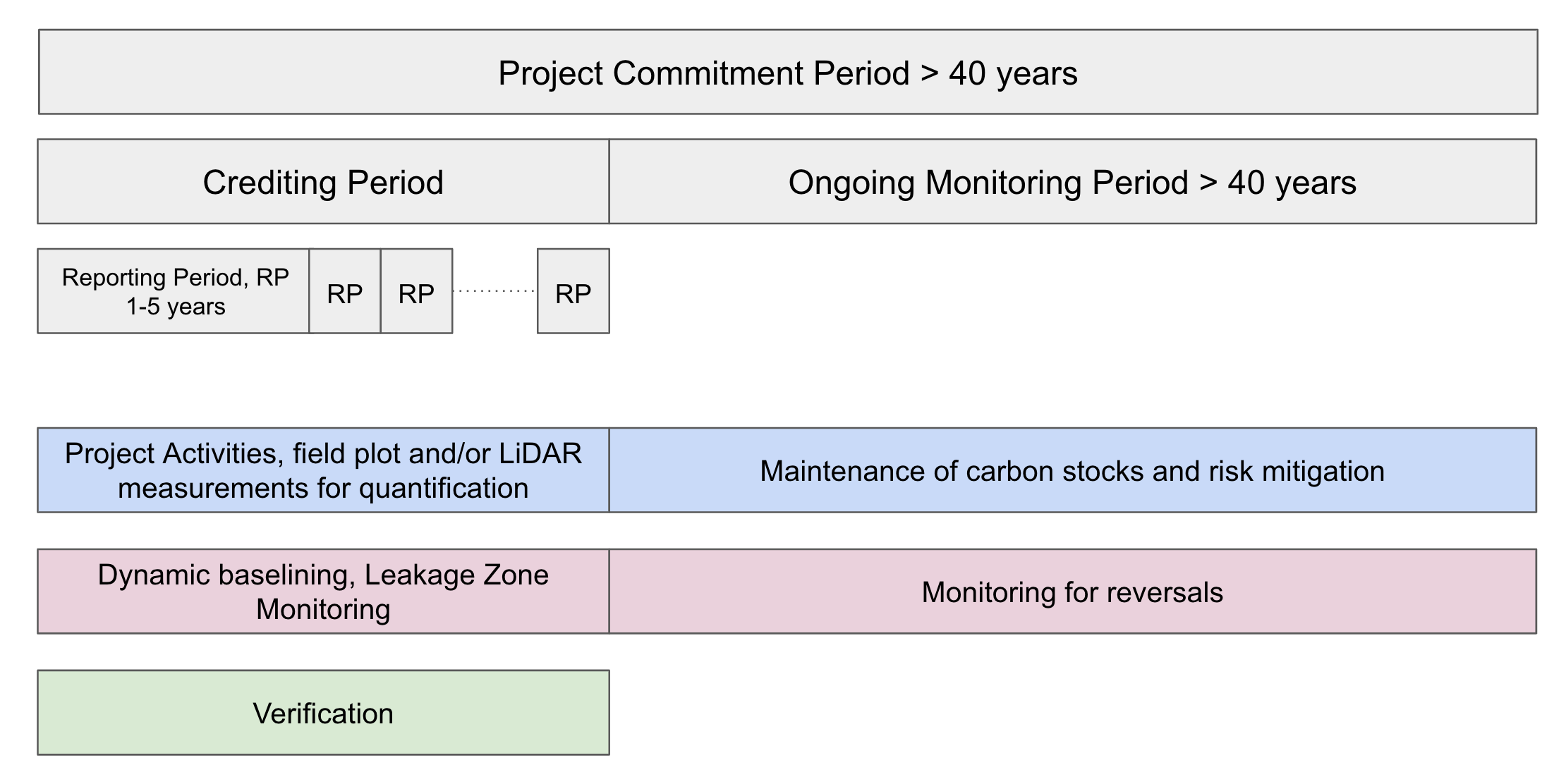
Figure 1 Summary of project periods. Colors represent actions owned by different stakeholders. Blue = Project Proponent. Green = VVB. Pink = Isometric.
5.6
Example Project Timeline
A project starting in 2025 has a Project Commitment Period of 100 years composed of a 40 year Crediting Period followed by 60 year Ongoing Monitoring Period. Credits issued have a 60+ year durability. Monitoring for quantification is conducted by the Project Proponent through the Crediting Period, and the reported activities are verified by a Validation and Verification Body (VVB) for each Reporting Period. At the end of the Crediting Period, maintenance of carbon stocks and monitoring for Reversals occurs for the remaining 60 years of the Project Commitment Period.
6.1
Overarching Principles
Following the Isometric Standard, Credits issued under this Protocol are contingent on the implementation, transparent reporting, and independent Verification of comprehensive safeguards. These safeguards encompass a wide range of considerations, including environmental protection, social equity, community engagement, and respect for cultural values. The process mandates that safeguard plans be incorporated into all major project phases, with detailed reports made accessible to stakeholders. Adherence to and verification of environmental and social safeguards is a condition for all Crediting Projects.
An environmental and social risk assessment in adherence with Section 3.7 of the Isometric Standard must be completed to identify potential risks, followed by the development of tailored mitigation plans. These plans must encompass specific actions to avoid, minimize or rectify identified impacts. Effective implementation of these measures must also be accompanied by a robust monitoring plan to detect adverse effects and pause project activities if necessary, using the principles of adaptive management described below.
Environmental and social risk identification, assessment, avoidance, and mitigation planning will be unique to the technical, environmental, and social contexts of The Project. To accommodate this variation, the requirements outlined in this section serve as a minimum to which the Project Proponent and Isometric can add risks on a case by case basis, to be included in the PDD, if applicable.
6.1.1
Governance and Legal Framework
Project Proponents must comply with all national and local laws, regulations and policies, and receive any necessary permits for project activities, if applicable. Where relevant, projects must comply with international conventions and standards governing human rights and uses of the environment.
Project Proponents must document activities that trigger environmental permitting requirements.
6.2
Adaptive Management
Adaptive management incorporates learnings and takeaways from project monitoring into project development11. Regular data collection and sharing is necessary to implement adaptive management. Results from data collection at the end of each Reporting Period must be shared with local stakeholders, as described in Section 6.5.1 of this Protocol, and be used to inform future iterations of project management and development.
Project Proponents are required to predict and plan for potential unintended outcomes of project activities and construct mitigation plans for such instances. Foreseeable risks identified during the preparation of the environmental and social risk assessment must be included in the PDD and the following must be detailed for each potential risk:
- A region specific mitigation plan
- The measured or observed outcome that will trigger the mitigation plan
- Plan for information sharing
- Emergency response plan, if applicable
The Project should not hinder the ability of the community or local ecosystem to adapt to climate change as a result of the CDR activity.
6.3
High Conservation Values
The High Conservation Values (HCV) Approach, developed by the HCV Network, identifies regionally specific facets of local communities and ecologies that must be considered during project developments resulting in land use change. The HCV Network has identified six values that may be at risk as a result of land use change projects. The values, along with corresponding requirements for Project Proponents to uphold them, are listed below:
- Species Diversity: Rare, threatened, endangered, or endemic species, at populations significant to regional, national, or global levels.
- Requirements. Population density of these species in the project area must not decrease as a result of project activities (see Section 6.3.1). It is recommended that Project Proponents strive to increase the populations of these species during project activities to improve the climate adaptation potential of the local ecosystem, which in turn increases the durability of carbon stored in aboveground biomass.
- In cases where reforestation will lead to a decrease in the population of rare, threatened, or endangered species which occupy non-forested or degraded lands, The Project may proceed if permitted by law and after a mitigation plan is developed in consultation with Isometric and included in the PDD. Mitigation plans must ensure no decrease in population density and should include activties such as:
- Relocation of population to areas within the same region as the project area, which can support and maintain the species' population;
- Maintenance of population in the project area through the development of ecologically appropriate reserves and wildlife corridors;
- Active monitoring plans.
- In some instances, endemic species may be overpopulated prior to project initiation and decrease as a result of project activities. These or similar situations may be allowable under this Protocol, in consultation with Isometric. Project Proponents must demonstrate that a population decrease in the project area will not adversely impact the species' metapopulation and that an endemic species was overpopulated in the project area through one of the following:
- Peer-reviewed scientific literature;
- Authoritative national- or regional-body publications; or
- A population census conducted by an independent third party in consultation with Isometric.
- In cases where reforestation will lead to a decrease in the population of rare, threatened, or endangered species which occupy non-forested or degraded lands, The Project may proceed if permitted by law and after a mitigation plan is developed in consultation with Isometric and included in the PDD. Mitigation plans must ensure no decrease in population density and should include activties such as:
- Requirements. Population density of these species in the project area must not decrease as a result of project activities (see Section 6.3.1). It is recommended that Project Proponents strive to increase the populations of these species during project activities to improve the climate adaptation potential of the local ecosystem, which in turn increases the durability of carbon stored in aboveground biomass.
- Landscape-level ecosystems, ecosystem mosaics and intact forest landscapes: Broad-scale regions of interacting ecosystems which contain species in their natural patterns or distributions at populations significant on regional, national, or global scales.
- Requirements. Ecological integrity in the project area must be maintained throughout project activities.
- Ecosystems and habitats: Rare, threatened, or endangered ecosystems or habitats.
- Requirements. Rare, threatened, and endangered ecosystems and habitats in the project area must be maintained and protected throughout project activities.
- Ecosystem services: Fundamental ecosystem functions critical to ecological integrity and life, e.g., oxygen production, water filtration and protection of catchments, soil formation and erosion prevention, temperature regulation, nutrient cycling, habitat formation, provisioning of food and forage for fauna, etc.
- Requirements. Ecosystem services should be restored to those rendered by forests within the project area region and maintained throughout project activities.
- Community needs: Commodities, resources, and community functions that are necessary for the livelihoods of local communities and Indigenous Peoples. This may include food, water, and infrastructure sources.
- Requirements. Community needs must be identified in consultation with local stakeholder groups. Community needs must not be damaged as a result of project activities. Access to community resources must not be limited as a result of project activities.
- Cultural values: Sites, landscapes, and habitats of significant cultural, historical, religious, economic, or archaeological value to local communities, Indigenous Peoples, or other groups identified to engage in those locations.
- Requirements. Cultural values must be identified in consultation with local stakeholder groups. Cultural values must not be damaged as a result of project activities.
For each value above, the Project Proponent must identify in the PDD if the value is present or absent in the project area. This list must be constructed in consultation with relevant stakeholder groups, as identified in Section 6.5.1 and carried out in accordance with Section 3.5 of the Isometric Standard . The Stakeholder Engagement Plan for HCV identification must also be included in the PDD.
If a value is absent from the project area, the Project Proponent must provide an explanation or justification such as survey results or recent publications. If a value is present in the project area, the Project Proponent must include a plan to monitor and protect it throughout the Project Commitment Period in the PDD. We encourage Project Proponents to review the Common Guidance for the Management and Monitoring of HCV in developing this plan. If protection is not feasible during the project activities and an HCV is damaged as a result of project activities, the Project Proponent must provide a restoration plan to return the area to its prior condition and quality.
If an HCV is threatened or damaged by forces or parties outside of the Project Proponent’s jurisdiction and not as a result of or response to project activities, the Project Proponent must report such instances to Isometric, but may not be responsible for enacting a restoration plan. Failure to properly identify, monitor, and protect an HCV may result in the cessation of Credits.
6.3.1
Rare, Threatened, and Endangered Species
The Project Proponent must provide due diligence to ensure that the population density of rare, threatened, and endangered species in the project area does not decrease, nor are new species added to this list, as a result of project activities. If either of these adverse impacts do occur, the Project Proponent must work with Isometric and the VVB to identify sources and explanations for these impacts in order to rule out project activities as the primary cause.
It is recommended that Project Proponents strive to increase the population of rare, threatened, and endangered species. Endangered species are defined as species under threat of extinction from all or a significant amount of their natural habitat. Threatened species are defined as those that are at risk of becoming endangered. Rare species are defined as those uncommon and found in isolated geographical locations. Project Proponents must consult local authorities for further regulations on these or similar groups. If local regulations exist, the Project Proponent must state them in the PDD.
The Project Proponent must consult reputable and current sources on rare, threatened, and endangered species to develop a list of these species, in the following order of priority:
- Local and/or regional registries;
- National registries;
- Peer-reviewed publications; and
- The International Union for Conservation of Nature (IUCN) Red List of Threatened Species14.
- For the purposes of this Protocol, the IUCN Red List designation of Vulnerable (VU) shall be considered Threatened, and Near Threatened (NT) shall be considered Rare.
The results of the rare, threatened, and endangered species list review must be included and referenced in the PDD.
For each rare, threatened, or endangered species identified, the Project Proponent must list the following in the PDD:
- Ecosystem services vital to the ecology and population stability of the rare, threatened, or endangered species found in the project area.
- How The Project will maintain or enhance these ecosystem services so as to promote the survival of the rare, threatened, or endangered species.
- A population monitoring plan. We encourage Project Proponents to consult Isometric, external subject matter experts, and/or authoritative resources in developing their plan.
The Project Proponent must handle data and information related to rare, threatened, and endangered species with discretion for the protection of these species, especially regarding species and/or regions that have histories of poaching, over-harvesting, or other elevated threats to population density and livelihoods.
6.4
Safeguarding of Biodiversity
As stated in Section 4.1, reforestation projects must occur on degraded land to be eligible for crediting under this Protocol. Because of this applicability requirement and the nature of reforestation projects to plant and maintain species in the project area, reforestation projects are well placed to increase biodiversity in the region. To benchmark increased biodiversity, Project Proponents must include more than five species from two or more genera in their planting plan and should prioritize the planting of endemic, rare, threatened, and endangered native species. Species should be planted at ecologically appropriate richness and evenness15. There may be some regions that naturally support a limited number of species that fulfill ecosystem services and other functions or indicators of healthy ecosystems. Project Proponents in these regions may deviate from the minimum required species and genera included in planting plans, in consultation with Isometric. Such deviations must be accompanied by appropriate documentation, based in scientific literature and/or ongoing field studies, in the PDD.
The tree species used for reforestation must follow the principles outlined below.
6.4.1
Species Selection for Reforestation
The Project Proponent must list the species planted and/or maintained in the project area via project activities in the PDD. These species may include native, naturalized, or non-native range-expanding species. Project Proponents must not introduce species invasive to the region or similar climates, geographies, or ecosystems of the project area16, 17. The definition of 'invasive species' in this Protocol is consistent with the Convention on Biological Diversity's definition of Invasive Alien Species, being a "species whose introduction and/or spread threaten[s] biological diversity"18. Projects that plant invasive species will not be eligible for crediting under this Protocol. Additionally, Project Proponents must not introduce any species that harm rare, threatened, or endangered species as defined in Section 6.3.1 or adversely impact the integrity of rare, threatened, or endangered ecosystems and habitats (see Section 6.3). Project Proponents are highly encouraged to consult with Isometric, the VVB, and/or external subject matter experts to ensure that species included in the reforestation plan meet these requirements and the criteria described below.
For the purposes of this Protocol, native species are defined as:
- Species indigenous to the project area that would be found naturally (not planted or introduced anthropogenically via assisted migration) in the project area prior to deforestation or degradation, and/or species that are indigenous to and found naturally in land adjacent to the project area; or
- Species indigenous to the region that have not grown in the project region for the past 100+ years due to displacement via anthropogenic factors or competition from invasive species, but are still well suited to the climate of the project area, as demonstrated by scientific literature, presence of these species in similar climates, and/or evidence of displacement via one of these two forces.
- Indigenous species that have not existed in the project region for the past 100+ years due to failure to adapt to changing climatic conditions may not be suitable for reintroduction for the purposes of GHG removal, but may be suitable for other ecosystem benefits. Reintroduction of such species should be done in consultation with Isometric.
Naturalized species are defined as:
- Species which occur in the project region at the time of project initiation, have existed in the project region for 100+ years, and have not threatened biodiversity in the region during that time frame, regardless of indigeneity.
Reforestation with native species should be the first course of action. If reforestation with only native and naturalized species is not feasible, non-native range-expanding species may be included in the reforestation planting plan. Any non-native species not considered range-expanding for the purposes of this Protocol must not be planted. Non-native range-expanding species are defined as:
- Species whose natural boundaries are expected to overlap with the project area by the end of the project lifetime and would naturally migrate to and occur within the project boundaries without human-intervention; or
- Species that currently exists in the same RESOLVE terrestrial biome8 as the project area, and where peer-reviewed literature or government agency documentation supports the species assisted migration as an adaptation response to climate change, and where such migration is projected to occur naturally over time due to climate change.
In such instances, the majority of species planted must be native and/or naturalized, and the plurality must be native species. Additionally, the following due diligence must be taken when planting non-native range-expanding species for a project to be eligible for crediting. The Project Proponent must demonstrate:
- Reforestation with native species will hinder the Project Proponent’s ability to meet project objectives:
- Introduction of native species will lead to negative ecosystem impacts.
- Native species will fail to thrive and contribute significantly to the carbon stock over the course of the Reporting Period. This may occur if the species lack climate resilience, marked by increased vulnerability to temperature fluctuations, changes in water availability, competition from invasive species, disease, etc.
- Reforestation via non-native range-expanding species will bring net positive ecosystem or community impacts that could not otherwise be achieved.
- Non-native range-expanding species are expected to serve as pioneer species for successional planting of native species, as demonstrated in scientific, peer-reviewed literature and/or in other reforestation projects in the same or similar regions.
Alternative burdens of proof may be sufficient, in consultation with Isometric.
The following due diligence must be conducted and included in the PDD if non-native range-expanding species are to be planted during project activities. The Project Proponent must demonstrate:
- The species are able to adapt to climate-induced changes expected to take place in the region over the project lifetime.
- The species will serve similar ecological niches as native and/or naturalized species present in the region at the time of project initiation (e.g., as a suitable food source for local fauna).
- The species do not have the potential to be invasive. This must be demonstrated through recent peer-reviewed literature and observational studies of the species in the same region and/or other regions with similar climates, geographies, and ecologies.
6.4.2
Seedling and Germplasm Pipeline
A robust seedling and germplasm pipeline is central to the ecological, socioeconomic, and cultural success of a reforestation project. A diverse, local, and sustainable pipeline ensures that project activities contribute to the restoration of ecosystem function and integrity, restore and protect biodiversity, safeguard community livelihoods, and uphold cultural values.
Project Proponents must procure and maintain their seedling and germplasm pipeline in alignment with the environmental and social safeguards outlined in Section 6 of this Protocol and Section 3.7 of the Isometric Standard.
The pipeline must be described in the PDD and the Project Proponent should:
- Procure genetically diverse seedlings and germplasms, sourced from within or near the project region. This conserves locally adapted traits and strengthens resilience to climate change, pests, and diseases.
- Prioritize sourcing from nurseries that employ local community members and align with the requirements and suggestions of Section 6.5: Safeguarding of Community Livelihoods, thereby generating equitable economic opportunities and fostering long-term community investment in project success.
- Stock and maintain sufficient germplasm resources to support not only forest regeneration, but also essential non-reproductive ecological functions such as nutrient cycling and faunal sustenance.
6.5
Safeguarding of Community Livelihoods
6.5.1
Stakeholder Engagement
In accordance with Section 3.5 of the Isometric Standard, Project Proponents must demonstrate active stakeholder engagement throughout project planning and operation, ensuring that all risk mitigation strategies contribute to sustainable project outcomes. Local stakeholders may contribute an in-depth understanding of the project area and operations, and provide invaluable insights and recommendations on potential risks, necessary safeguards and specific monitoring needs. Engaging local stakeholders in reforestation projects creates community buy-in, providing long term commitment and investment in the success of reforestation projects19, 11. Furthermore, lack of community support, stakeholder engagement, and perceived community benefits has been identified as a primary source of project failure in previous forestry projects20.
The Project Proponent must develop a Stakeholder Engagement Plan in accordance with the requirements outlined in Section 3.5 of the Isometric Standard. The plan and supporting documentation, including evidence of meetings or other forms of engagement, must be submitted in the PDD.
Prior to the commencement of project activities, Project Proponents are required to assess if Indigenous Peoples will be impacted by project activities, in consultation with Isometric. Impacts may include, but are not limited to:
- Project activities that occur on land or territories that is owned, occupied, or utilized by Indigenous Peoples, regardless of whether or not this claim is recognized by the local governing body or held by rights to self-determination, as recognized by the United Nations;
- Project activities that will affect natural resources necessary for the livelihoods or cultural rights of Indigenous Peoples.
Project Proponents must consult a reputable third party or subject matter expert to assess if Indigenous Peoples will be impacted by project activities. The results of this report must be included in the PDD. If the report identifies potential impacts to Indigenous Peoples, the Project Proponent must enact a Stakeholder Engagement Plan consistent with the principles of Free, Prior, and Informed Consent (FPIC) as outlined by the United Nations (UN) Declaration on the Rights of Indigenous Peoples21 in 2007 and expanded upon by the Food and Agriculture Organization of the United Nations in 201622.
- Free: Stakeholders are not subject to intimidation, coercion or manipulation during the decision making process.
- Prior: Engagement is sought in the early stages of project development before commencement of project activities. Consent must be sought as part of project development, regardless of local requirements. The timeline for the decision making and deliberation periods is set in consultation with all stakeholder groups and is informed by customary, local, and/or traditional practices.
- Informed: Information is presented in a manner that is accessible to all stakeholder groups. Accessible content may differ across stakeholder groups. The Project Proponent must consider in the information sharing process the language and medium of communication. For example, if information is presented electronically, stakeholders must have access to and familiarity with the necessary technology to review the information. If information is presented during in-person meetings, the meetings must be held at a time and in a location that is conducive to stakeholder attendance. Information presented to stakeholders must be objective and present trade-offs fairly and accurately. Finally, information must be provided on an ongoing basis. The following due diligence is strongly recommended to ensure stakeholder groups are well informed of project development and outcomes:
- Stakeholders should be made aware of the value of the Credits, and anticipated revenue of The Project at-large. The Project’s anticipated growth and issuance should be modeled, and simulations describing the value of Credits at current market prices should be made clear to proponents.
- Stakeholders should have full access to the project’s finances, budget, and forecasted returns.
- Stakeholders should be aware of alternative land-use scenarios.
- Stakeholders should be aware of the value of the timber on The Project once the Crediting Period nears an end, so that they can better commit to conservation and upholding the contract.
- Stakeholders should have a clear understanding of the breakdowns in project income expenditure, and a clear understanding of the precise percentage of revenue that they are entitled to.
- Consent: Must be freely given and may be withdrawn. Consent may be conditional upon milestones in project development or the emergence of new information. Stakeholder consent is not guaranteed as a result of the Stakeholder Input Process. Consent must be reached by 75% of adults belonging to the stakeholder group.
The Project Proponent is encouraged to prepare alternatives for the withdrawal or denial of consent to project activities by stakeholder groups.
If required, the stakeholder engagement process must be enacted early in the project development process, prior to the initiation of project activities. The stakeholder engagement schedule must be circulated prior to project initiation, and with enough notice to engage stakeholders in the planning processes. In some instances, Project Proponents that initiated project activities prior to engaging with Isometric and did not engage Indigenous Peoples stakeholders under the principles of FPIC may still be eligible for crediting under this Protocol, in consultation with Isometric, by demonstrating how stakeholder engagement will be incorporated into future project planning.
The following may serve as burdens of proof that the Stakeholder Input Process conforms with the principles of FPIC. The Project Proponent must indicate how these steps in the stakeholder engagement process were or will be carried out during the project lifetime. Multiple rounds of stakeholder engagement may take place during a project lifetime, as needed. The Project Proponent may identify other burdens of proof demonstrating that the principles of FPIC have been observed and submit them in the PDD in addition to, or instead of, those below, in consultation with Isometric.
- Measures taken to effectively reach (i.e., identify and locate) all stakeholder groups. If the Project Proponent is not able to reach all adult community members, the percentage of adults in the community reached must be included in the PDD, as well as proof of the attempt to reach the remaining community members. The majority of adult community members must be successfully reached to be eligible for crediting under this Protocol.
- The manner in which information was presented to stakeholders, including the medium and language.
- How stakeholder input was obtained, including the medium and language.
- How stakeholder input was incorporated into the project design.
The VVB may conduct random surveys or interviews with stakeholder groups, and/or witness some or all of the processes described above.
Project Proponents that do not identify Indigenous Peoples that will be affected by project activities are encouraged to consider if other relevant stakeholders rely on land or resources located within the project area, and engage them following the principles of FPIC described above. All stakeholder groups and local communities have valuable and unique perspectives on developments in the project area, which can contribute to project success.
The following information from the stakeholder engagement process must be made publicly available, with personal information anonymized or redacted to protect stakeholders, project personnel, and project outcomes. This may include:
- Due diligence that the FPIC processes were carried out (e.g., meeting recordings or copies of information shared with stakeholders)
- Budget reports, including revenue sharing agreements
6.5.2
Community Impacts and Well-being
6.5.2.1
Community Well-being
The Project Proponent must identify and develop processes for the protection and promotion of community well-being in the PDD, as follows:
- Protection of human rights:
- Policies and practices upholding anti-discrimination on the basis of gender, sexual orientation, etc.
- Grievances, feedback, and complaints:
- The process by which the Project Proponent accepts grievances, feedback, and complaints. Project Proponents must consult a third party to address grievances. The grievance redress process must be outlined in the PDD.
- Mediation and resolution process for grievances and complaints.
- Employment Opportunities:
- Hiring practices and policies, including the number of short-, medium-, and long-term employment opportunities that were recruited for in the local community relative to total new jobs created.
6.5.2.2
Community Impacts
As previously mentioned, community buy-in is critical to the success of a reforestation project 19 , 11 , 20. Community buy-in may be established when stakeholders are properly informed about the benefits they can expect from the reforestation project. Equally important in maintaining buy-in is for the positive impacts resulting from the project to match the (perception of) potential benefits presented to community stakeholders at the project onset. A mismatch in benefits expected and benefits realized may similarly hinder project success.
While this Protocol will not prescribe requirements for community impacts, the Project Proponent is strongly encouraged to consider establishing the following programs and activities:
- Employment opportunity programs favoring local community members, especially in the creation of long-term jobs;
- Establishment of community benefit-sharing arrangements;
- Construction of infrastructure, such as roads, that are accessible to the community;
- Development of site specific mitigation plans for potential negative community impacts.
Positive impacts should be felt by all stakeholder groups identified in Section 6.5.1. Project Proponents should consider which groups may face the brunt of negative community impacts, and how positive community benefits may be shared equitably with these and other marginalized groups.
It is recommended that the Project Proponent provide support to the local communities and ecosystems to establish region specific mitigation strategies to adapt to changing climates.
7.0
Relation to Isometric Standard
The following topics are covered briefly in this Protocol due to their inclusion in the Isometric Standard, which governs all Isometric Protocols. See in-text references to the Isometric Standard for further guidance.
7.1
Project Design Document
For each specific project to be evaluated under this Protocol, the Project Proponent must document project characteristics in a Project Design Document (PDD) as outlined in Section 3.2 of the Isometric Standard. The PDD will form the basis for project Validation and evaluation in accordance with this Protocol.
7.2
Verification and Validation
Projects must be validated and net CO2e removals verified by an independent third party, consistent with the requirements described in this Protocol, as well as in Section 4 of the Isometric Standard.
The Validation and Verification Body (VVB) must consider the following requisite components:
- Verify that The Project meets the Applicability conditions described in Section 4
- Verify that the Environmental & Social Safeguards outlined in Section 6 are met
- Verify that the System Boundary & Leakage assessment adheres to the requirements of Section 8
- Verify that the quantification approach and monitoring plan adheres to requirements of Section 9
- Verify that the conditions for ensuring durability and monitoring for Reversals in Section 10 are met
- Verify that The Project is compliant with requirements outlined in the Isometric Standard
7.2.1
Verification Materiality
The threshold for Materiality, considering the totality of all omissions, errors and misstatements, is 5%, in accordance with Section 4.3 of the Isometric Standard.
Verifiers should also verify the documentation of uncertainty of the GHG Statement as required by Section 2.5.7 of the Isometric Standard. Qualitative Materiality issues may also be identified and documented, such as:
- Control issues that erode the verifier’s confidence in the reported data;
- Poor management documented information;
- Difficulty in locating requested information; and
- Noncompliance with regulations indirectly related to GHG emissions, removals or storage
7.2.2
Site Visits
Project Validation and Verification must incorporate site visits to project facilities, namely in situ field plots, in accordance with the requirements of ISO 14064-3, 6.1.4.2. This is to include, at a minimum, site visits to the project site during Validation and initial Verification. Validators should, whenever possible, observe project operations to ensure full documentation of process inputs and outputs through visual observation (see Section 4 of the Isometric Standard).
Additional site visits may be required if there are substantial changes to field operations over the course of Validation, or if deemed necessary by Isometric or the VVB. Site visit plans are to be determined according to the VVB’s internal assessment, in consultation with Isometric.
7.2.3
Verifier Qualifications & Requirements
Verifiers and Validators must comply with the requirements defined in Section 4 of the Isometric Standard. In addition, verification teams must maintain and demonstrate expertise associated with the specific technologies of reforestation and forest management, including both forest field measurements and Earth System remote sensing data processing and analysis.
7.3
Ownership
CDR via reforestation is a result of a multi-step process (e.g., seed planting, forest maintenance, monitoring), with activities in each step potentially managed by a different operator, company, or owner. A single Project Proponent must be specified contractually as the sole owner of the Credits when there are multiple parties involved in the process, and to avoid Double Counting of net CO₂e removals. Contracts must comply with all requirements defined in Section 3.1 of the Isometric Standard.
7.4
Additionality
The Project Proponent must be able to demonstrate additionality through compliance with Section 2.5.3 of the Isometric Standard. The Baseline scenario and Counterfactual utilized to assess additionality must be project-specific and comply with Section 9.4 of this Protocol.
Government subsidies or civil contractual obligations for reforestation, such as organization bylaws, inhibit additionality and fall under the Regulatory criteria in Section 2.5.3 of the Isometric Standard. Environmental additionality is assessed each Reporting Period using dynamic baselining as outlined in Section 9.4.
Additionality determinations should be reviewed and completed at every Verification at a minimum, or whenever project operating conditions change significantly, such as the following:
- Regulatory requirements or other legal obligations for project implementation change or new requirements are implemented;
- Project financials indicate Carbon Finance is no longer required to operate the Project, potentially due to, for example:
- sale of non-timber co-products that make the business viable without Carbon Finance; or
- reduced rates for capital access.
If a review indicates The Project has become non-additional, The Project will be ineligible for future Credits. Current or past Crediting Periods will not be affected.
7.5
Uncertainty
The uncertainty in the overall estimate of the net CO2e removal as a result of The Project must be accounted for. The total net CO2e removed for a specific Reporting Period, , , must be conservatively determined in accordance with the requirements outlined in Section 2.5.7 of the Isometric Standard.
7.5.1
Reporting of Uncertainty
Projects must report a list of all key variables used in the net CO2e removal calculation and their uncertainties, as well as a description of the uncertainty analysis approach, including:
- field measurements used for the net CO2e removal calculation
- parameters that impact the estimation of the total aboveground woody biomass, such as allometric equation parameters, canopy height, etc.
- parameters used for calculating carbon stocks, including root-to-shoot ratios and carbon fractions
- quantification of aboveground biomass (AGB) model strength through comparison with independent datasets
- emission factors utilized, as published in public and other databases used
The uncertainty information should at least include the minimum and maximum values of a variable. More detailed uncertainty information should be provided if available, as outlined in Section 2.5.7 of the Isometric Standard.
In addition, a sensitivity analysis that demonstrates the impact of each input parameter’s uncertainty on the final net CO2e uncertainty must be provided. Details of the sensitivity analysis method must be provided such that a third party can reproduce the results. Input variables may be omitted from an uncertainty analysis if they contribute to a < 1% change in the net CO2e removal. For all other parameters, information about uncertainty must be specified.
7.6
Data Sharing
In accordance with the Isometric Standard, all evidence and data related to the underlying quantification of CO₂e removal and environmental and social safeguards monitoring will be available to the public through the Isometric platform. That includes:
- Project Design Document
- See Section 11 for a list of pre-deployment requirements that must be included in the PDD
- GHG Statement
- Measurements taken, with supporting documentation (e.g., calibration certificates)
- Emission factors used
- Scientific literature used
- Proof of approval for necessary permits
- Remote sensing and field plot data collected by The Project
- All maps generated for calculating carbon stocks in the project area
- All maps generated for calculating carbon stocks in control areas (geospatial reference data can be removed for privacy reasons)
- Model specifications and output
The Project Proponent can request certain information to be restricted (only available to authorized Buyers, the Registry, and VVB) where it is subject to confidentiality. This includes emission factors, specific data, and/or proprietary models from licensed databases. However, all other numerical data produced or used as part of the quantification of net CO2e removal will be made available.
8.0
System Boundary, Leakage and Project Baseline
8.1
Systems Boundary and GHG Emissions Scope
The scope of this Protocol includes GHG sources, sinks and reservoirs (SSRs) associated with a reforestation project. A cradle-to-grave GHG Statement must be prepared encompassing the GHG emissions relating to the activities outlined within the system boundary.
Any emissions from sub-processes or process changes that would not have taken place without The Project, and any activity that ultimately leads to the issuance of Credits, must be considered in the system boundary. This allows for accurate consideration of additional, incremental emissions induced by The Project.
The system boundary must include all SSRs controlled by, and related to, The Project, including but not limited to the SSRs in Table 1. If any GHG SSRs within Table 1 are deemed not appropriate to include in the system boundary, they may be excluded, provided that robust justification and appropriate evidence is included in the PDD. Materiality considerations for exclusions are set out in Section 8.1.1.1.
Table 1. Scope of activities and GHG SSRs to be included in the system boundary.
| Activity | GHG Source, sink or Reservoir | GHG | Scope | Timescale of emissions and accounting allocation |
|---|---|---|---|---|
| Project Establishment | Equipment and materials | All GHGs | Embodied emissions associated with equipment and materials manufacture related to project establishment (lifecycle modules A1-323). This must include product manufacture emissions for:
| Before project operations start - must be accounted for in the first Reporting Period or amortized in line with allocation rules (see Section 9.5.1) |
| Equipment and materials transport to site | All GHGs | Transport emissions associated with transporting materials, equipment and seedlings to the project site(s) (lifecycle module A423). | ||
| Planting and installation | All GHGs | Emissions related to construction and installation of the project site(s) (lifecycle module A523). This must include, as appropriate:
Emissions associated with soil disturbance are excluded as emissions are likely to be balanced by soil carbon accumulation over the project lifetime. Soil carbon is not included as part CO2 stored due to uncertainties. Projects should limit soil inversions during project establishment to < 25 cm (See Section 4.4). | ||
| Misc. | All GHGs | Any SSRs not captured by categories above (e.g., staff travel). | ||
| Operations | Fertilizer use (Direct) | N2O | Direct emissions related to the use of nitrogen-based fertilizers. | Over each Reporting Period - must be accounted for in the relevant Reporting Period (see Section 9.5.2). |
| Forest management | All GHGs | Emissions related to forest management activities (e.g., pruning, weeding, pest control, biomass burning and watering). This must include embodied emissions of equipment, as well as consumables such as water, fertilizers and pesticides. | ||
| Maintenance | All GHGs | Maintenance of the project area, including any repair or replacement of equipment, vehicles, buildings and infrastructure. | ||
| All GHGs | Emissions related to MRV activities (e.g., measurements, sampling, or commissioning LiDAR flights). | |||
| CO2 stored | CO2 | The gross amount of CO2 removed and durably stored in living aboveground woody biomass and belowground woody biomass (see Section 9.3). | ||
| Misc. | All GHGs | Any SSRs not captured by categories above (e.g., staff travel). | ||
End-of-Life | Ongoing Monitoring | All GHGs | Emissions relating to monitoring activities over the Project Commitment Period. | After Reporting Period - must be estimated and accounted for in the first Reporting Period or amortized in line with allocation rules (see Section 9.5.3) |
| Ongoing Forest management | All GHGs | Emissions relating to ongoing project management activities over the Project Commitment Period. | ||
| Misc. | All GHGs | Any SSRs not captured by categories above (e.g., ongoing staff travel). |
The Project Proponent must consider all GHGs associated with SSRs, in alignment with the United States Environmental Protection Agency’s definition of GHGs, which includes: carbon dioxide (CO2), methane (CH4), nitrous oxide (N2O) and fluorinated gasses such as hydrofluorocarbons (HFCs), perfluorocarbons (PFCs), sulfur hexafluoride (SF6) and nitrogen trifluoride (NF3). For CO2 stored, only CO2 will be included as part of the quantification and for Fertilizer use (Direct), only N2O shall be included as part of the quantification. For all other activities, all GHGs must be considered. For example, the release of CO2, CH4, and N2O is expected during diesel combustion.
All GHGs must be quantified and converted to CO2e in the GHG Statement using the 100-year Global Warming Potential (GWP) for the GHG of interest, based on the most recent volume of the IPCC Assessment Report (currently the Sixth Assessment Report24).
Miscellaneous GHG emissions are those that cannot be categorized by the GHG SSR categories provided in Table 1. The Project Proponent is responsible for identifying all sources of emissions directly or indirectly related to project activities and must report any outside of the SSR categories identified as miscellaneous emissions.
Emissions associated with The Project's impact on activities that fall outside of the system boundary of The Project must also be considered. This is covered under Leakage in Section 8.3.
8.1.1
System Boundary Considerations
8.1.1.1
Materiality
Some studies25, 26 have identified reforestation projects to have high removal efficiency, with lower emissions on average when compared to removal capacity, than other CDR pathways. These studies also indicate that emissions associated with reforestation projects still make up a material fraction of net CDR for these projects. Studies27 also highlight that other existing methodologies vastly underestimate emissions associated with reforestation projects, therefore leading to a risk of over-crediting.
At the time of Protocol development, a lack of suitable benchmark data exists to exclude categories of SSRs from GHG accounting requirements. When a suitable range of appropriate project data is available, this will be revisited. In the meantime, a Materiality threshold has been set at 1% of total removals. If emissions for an SSR are expected to be < 1% of total removals, they may be excluded from the GHG systems boundary. A sensitivity analysis must be used to demonstrate that excluded GHG SSRs are likely to contribute to < 1% of total project removals. The sensitivity analysis may be based on high level information and indicative values, but the decision making and logic followed must be appropriately and transparently evidenced. All exclusions must cumulatively make up < 1% of total removals. This threshold will be revised in light of new information or literature becoming available.
8.1.1.2
Ancillary Activities
Ancillary activities (such as supplementary research and development activities and corporate administrative activities) that are associated with The Project, but are not directly or indirectly related to the issuance of Credits, can be excluded from the system boundary.
8.1.1.3
Secondary Impacts on GHG Emissions
Reforestation may have additional impacts on GHG emissions beyond the scope of this Protocol. For example, positive leakage may occur where reforestation practices lead to positive ecological impacts outside of the project boundary. These potential secondary climate effects are not considered in this Protocol.
8.2
Project Baseline
The Baseline scenario for reforestation assumes that the activities associated with The Project do not take place and that any infrastructure associated with The Project is not built.
The Counterfactual is the CO2 stored that would have occurred due to natural regeneration over the Crediting Period in the absence of The Project. This Protocol uses a dynamic baseline approach to quantify the Counterfactual. This is detailed in Section 9.4.4.
8.3
Leakage
8.3.1
Overview of Leakage Assessment
Leakage emissions, , occur when project activities lead to emissions that occur outside the system boundary of reforestation projects. They include increases in GHG emissions as a result of reforestation projects displacing emissions or causing a secondary effect that increases emissions elsewhere. Three key types of leakage can occur for reforestation projects:
- Activity-shifting leakage. Reforestation projects may displace activities in their project areas, leading to an increase in those activities outside of the project area, which may result in potential land conversion. Examples are where the local community can no longer use the project site for subsistence, or where farmers are displaced as a result of project activities. This type of leakage is known as “Direct” leakage as the relevant stakeholders can be identified and the activity-shifting is traceable.
- Market leakage. Reforestation projects may displace activities, which results in a reduction in supply of a commodity. Changes to the supply and demand equilibrium causes other market actors to shift their activities, leading to potential land conversion. This type of leakage is known as “Indirect” leakage because its effects cannot be isolated and measured directly. Quantifying the likelihood and potential magnitude of market leakage is complex and relies heavily on modeling and available literature.
- Ecological leakage. Project activities may lead to emissions in areas outside of the project site as a result of ecological interactions, for example unintended hydrological impacts, introduction of disease, or secondary impacts of faunal influx.
Project activities that adversely alter the water table, harming ecological integrity within the project area and surrounding landscape and watershed, are not permitted under this Protocol. Furthermore, this Protocol limits reforestation to landscapes that were historically forests. Therefore, it is unlikely that surrounding landscapes sensitive to hydrological dynamics that were not present at the time the site was historically forested would have been established since deforestation. Assessing wider ecological leakage impacts is complex. For this version of the Protocol ecological leakage is assumed to be zero. This will be revisited in future updates to the Protocol.
Activity-shifting and market leakage are addressed in this Protocol. The overall process for addressing activity-shifting and market leakage is set out in the flowchart in Figure 2.

Figure 2 Flowchart of process for addressing activity-shifting and market leakage.
The flowchart is based on the following principles:
- If the commodity was used for subsistence this presents a risk of activity-shifting leakage.
- Activity-shifting leakage risk can be directly identified and mitigated.
- If the commodity was commercial, there is always a risk of market leakage.
- If the commodity was commercial, there might also be a risk of activity-shifting leakage.
- Where Direct Actors have been identified as impacted, activity-shifting leakage mitigation activities will address both activity-shifting leakage and market leakage. However, if only market leakage mitigation is implemented, this will not satisfy the activity-shifting leakage risk. For this reason, if only market leakage mitigation is undertaken, additional activity-shifting leakage monitoring must take place. If only partial or no leakage mitigation is in place, then the market leakage deduction must be applied, as well as a requirement for activity-shifting leakage monitoring.
- Where the commodity was used for subsistence and is not mitigated in full, The Project is not eligible. This is on the grounds of a very high risk of activity-shifting leakage due to dependencies on the land, but also because the project area was an area fundamental for the livelihoods of communities.
- Leakage mitigation has different requirements depending on whether it is addressing activity-shifting leakage or market leakage.
8.3.2
Pre-Project Information
Implementation of the flowchart in Figure 2 requires an understanding of Pre-Project Productivity, , including pre-project information about Direct Actors and how the commodity was used. Direct Actors are defined as site owners, tenants or other users that engaged with the project site in a way that produced commodities before the project activities commenced.
The information required is set out below:
- including the type of commodity and yield; and
- Whether the commodity was used for subsistence or commercial production.
- For the purposes of this assessment, commodities that are commercial, but primarily sold to the local community, are considered subsistence.
8.3.2.1
Determining Pre-Project Productivity,
is defined as the annual productivity of a commodity type at the project site in relevant units (e.g., tonnes/ yr). This should be an average of the three years prior to the project activities starting. For crops, this should be reflective of the last three complete annual crop cycles. For livestock, this should be reflective of the maximum cattle inventory over the last three years of production. For all other commodities, this should be reflective of production over the last three years of production.
The data hierarchy for obtaining information for is set out below:
- Farm records, including physical production records and accounts for crops, livestock, poultry and timber, and financial logs including income and expense records and receipts. Farm records may include traditional activity log data, or data from technology like smart tractors and GPS tags on cattle;
- Land registry data which details previous land holdings at the project site and production information related to land holdings;
- Remote sensing data which can be used to inform commodity production on land.
The hierarchy must be followed and data choices evidenced. For example, if land registry data is used, sufficient evidence of no available farm records will be required.
As part of determination of , the Project Proponent must confirm the following:
- The type of commodity, , that existed at the project site pre-project
- The productivity of commodity production,
8.3.2.1.1
Type of commodity,
The following considerations and assumptions should be made when determining the type of commodity, :
- Where land registry data is used to determine commodity type and commodities produced by one land holding are not quantified separately, or spatially separated, the most conservative assumption on commodity type for the site as a whole must be made. The most conservative assumption should be determined by running the calculations for (see Equation 5) assuming 100% of the production for each commodity and zero mitigation. The commodity that contributes to the highest value for should be assumed as full commodity production at the site.
- Where remote sensing data is used:
- Conservative assumptions on commodity type must be made in any areas of uncertainty. Any assumptions made must be transparently documented and justified.
- If the land use changed within the five years prior to the project start date, for example from arable use to pasture, the most recent commodity type should be used if it was in use for at least one year or one full crop rotation cycle.
- If more than one commodity type is identified, they must both be assessed as part of the leakage assessment provided that the spatial extent of each commodity type is clear.
8.3.2.1.2
Productivity of commodity production,
Productivity must be reflective of an average of the three years prior to the project activities starting.
The following considerations and assumptions should be made when determining productivity:
- Farm records must reflect the most recent relevant commodity or ownership class where estimates have been disaggregated by those attributes, and must be substantiated with a signed attestation from the farmer or landowner.
- Any assumptions made to interpret productivity data from farm records or land registry data must be of a conservative nature and be transparently reported.
- Methodologies that determine productivity data from remote sensing may be reviewed on a case by case basis. Models must be regionally- and commodity-appropriate and should have a minimum observation frequency of twice per year over a three-year period. Any inferences of productivity made using remote sensing data must be clearly referenced and justified. These must be of a conservative nature and be transparently reported. Future revisions of this Protocol will consider appropriate requirements for using remote sensing data to determine productivity as standard methodology.
- Where productivity related information is not available, average yield for the region may be used as a proxy for productivity. For example, annual yield data per state or region for the commodity type from the United States Department for Agriculture. An average over the last five years must be taken to account for anomalies.
- Where region-specific data is not available, average yield data at a national level may be used as a proxy for yield. For example, annual yield data for the commodity type from the Food and Agriculture Organization of the United Nations. An average over the last five years must be taken to account for anomalies.
- Where regional or national averages are not available for fuelwood production, average above-ground biomass growth rates published by the IPCC that are applicable to the region should be used.
8.3.2.2
How the Commodity was Used
The Project Proponent must determine the previous use of the commodity and whether it was:
- A commercial commodity: a commodity that is destined for regional, national, or global commercial markets; or
- A subsistence commodity: a commodity that is not destined for regional, national, or global commercial markets and is consumed by the local community.
The Project Proponent must determine this using the following information:
- An affidavit from the identified Direct Actors confirming the end-users of the commodity, or the majority buyer(s) the commodity was sold to. Direct Actors must include the previous site owners, tenants, or other users that engaged with the project site in a way that produced commodities.
- An affidavit from the local authority claiming that the project area was publicly owned and used for subsistence.
- An affidavit from members of the local community confirming that the project area was used for subsistence.
- An affidavit or records from local intermediaries such as wholesalers, distributors, food processors, grain elevators, or livestock auctions, confirming that they purchased commodities from the project site in the past.
If it is not possible to determine whether the commodity was for subsistence or commercial use, then the Project Proponent must assume it was subsistence.
8.3.2.3
Evidencing Zero Pre-Project Productivity
If The Project determines that is zero, this must be evidenced appropriately. This includes:
- Evidence of no farm records on open source sites;
- Land registry data which details no previous agricultural land holdings at the project site;
- Self-assessment from Direct Actors regarding prior use of the site, including photo evidence;
- Written confirmation from project site neighbors regarding the prior use of the site, including photo evidence. This may be land owners or managers from adjacent areas. Where possible this must include a diverse range of stakeholders.
Evidence must be provided for three years preceding the Project Proponent’s purchase of the site for reforestation, or the project start date, whichever is earlier.
In addition, Isometric will undertake remote sensing analysis on project sites which claim that is zero. Remote sensing mapping will be transparently displayed on the registry. Only where remote sensing analysis indicates there are no signs of agricultural production, pasture, or timber harvesting will The Project be eligible for claiming zero .
8.3.2.4
Calculation of CO2eLeakage
is part of the calculation of , as set out in Equation 21 in Section 9.5.
is quantified with the following equation:
(Equation 1)
Where:
- is the total emissions associated with leakage during the first Reporting Period, RP, in tonnes CO2e.
- is the total emissions associated with market leakage for a Reporting Period, RP, in tonnes of CO2e, see Section 8.3.5.
- is the adjustment to leakage emissions as a result of activity-shifting leakage being identified via monitoring for a Reporting Period, RP, in tonnes of CO₂e, see Section 8.3.6.2.
- is total emissions associated with leakage mitigation activities for a Reporting Period, RP, in tonnes of CO2e, see Section 8.3.4.
is quantified for every Reporting Period, however the following should be noted:
- is only estimated once during the first Reporting Period. The emissions associated with market leakage must be allocated to the first Reporting Period.
- is based on ongoing monitoring and therefore must be reported at every Verification. It is not reported during the first Reporting Period. For the first Reporting Period, and any preceding Reporting Periods where no activity-shifting leakage is identified, is zero. Activity-shifting leakage adjustments identified (up to a maximum of total possible leakage) should be allocated to the Reporting Period in which they are identified.
- must be allocated to the Reporting Period in which they occur. For example, emissions that occur as a result of establishment should be allocated to the first Reporting Period. Ongoing emissions, such as fuel use must be allocated to the Reporting Period in which they occur.
8.3.3
Leakage Mitigation
The aim of leakage mitigation activities is to reduce the amount of leakage by increasing production of the commodity elsewhere. Leakage mitigation must take place in areas called Leakage Mitigation Sites. These must be separate to the project site, but may be directly adjacent.
The following equation is used to calculate the effectiveness of leakage mitigation:
(Equation 2)
Where:
- is unmitigated Pre-Project Productivity, in appropriate units (e.g., tonnes per year).
- is Pre-Project Productivity - average annual production of commodity that would have been produced in the absence of The Project, in appropriate units (e.g., tonnes per year).
- = Mitigation area productivity, in appropriate units (e.g., tonnes per year).
When is 0, The Project had zero productivity.
When is > 0 and is 0, The Project has achieved full leakage mitigation and does not take a market leakage emissions deduction.
When is > 0 and is > 0, The Project takes a market leakage emissions deduction.
Leakage mitigation requirements are different depending on whether mitigation is to address market leakage (see Section 8.3.3.2) or activity-shifting leakage (see Section 8.3.3.1). Activity-shifting leakage will also by nature address market leakage, however market leakage alone will not address activity-shifting leakage.
In addition to the leakage type specific requirements, all leakage mitigation activities must meet the following requirements:
- A written agreement must be in place stating that the landowner of the Leakage Mitigation Site allows the Project Proponent to uniquely claim the increases in productivity as leakage mitigation associated with The Project. This must be covered via legal agreements for a five year term.
- Leakage mitigation activities must provide support to landowners of the Leakage Mitigation Site for a minimum of five years. This is on the basis that the initial leakage mitigation activity leads to sustainable recurring revenue for landowners of the Leakage Mitigation Site.
- Leakage mitigation may lead to increased productivity via creating new production on lands that were not previously used for production, or via intensifying production on existing production lands.
- Land selected for leakage mitigation must not have any other productivity that is negatively impacted by mitigation.
- The mitigation activity must lead to an increase in productivity as a direct result of intentional action from the Project Proponent.
- The spatial extent of the Leakage Mitigation Site and full details of activity must be provided as part of the PDD.
8.3.3.1
Activity-Shifting Leakage Mitigation
For mitigation of activity-shifting leakage, the Project Proponent must have a full understanding of the information set out in Section 8.3.2.1: Determining Pre-Project Productivity. The mitigation must be informed by the Direct Actors and be undertaken in agreement with Direct Actors. Mitigation activities must lead to new productivity or productivity increases that directly benefit the Direct Actors. This likely means that the increase in production should be limited to the same commodity type, but this decision should be informed by the Direct Actors. This also likely means that the Leakage Mitigation Site should be in the same locality, but again this should be informed by the Direct Actors.
The Project Proponent should engage with Direct Actors associated with the site’s prior productivity to understand how the project activity impacted the previous users of the project site. Direct Actors include the previous site owners, tenants or other users that engaged with the project site in a way that produced commodities.
The Project Proponent must receive an affidavit from the identified Direct Actors confirming the following:
- Their occupation;
- How they previously used or engaged with the project site;
- How the project activities impacted their use of the project site; and
- How they designed mitigation activities with the Project Proponent.
Full records of correspondence, including meeting notes, and signed agreements must be made available as part of the PDD.
If information from Direct Actors is unavailable, the Project Proponent will be unable to undertake activity-shifting leakage mitigation.
8.3.3.2
Market Leakage Mitigation
For mitigation of market leakage, the following must be true in addition to the requirements set out in Section 8.3.3:
- The mitigation may increase productivity of a substitute crop that comes under the same commodity category, as this will result in a land sparing effect.
- The Leakage Mitigation Site should be in the same region. If this is not possible, the Leakage Mitigation Site must be in the same national boundary.
8.3.4
Calculating the Emissions Impact of Leakage Mitigation Activities, CO2eLeakage Mitigation Emissions
The emissions impact of leakage mitigation activities, must be considered. The same system boundaries set out in Table 1 must be considered, noting that it is likely only certain GHG SSRs will be included. At minimum, the following emissions sources must be considered:
- Embodied Emissions associated with any new construction (e.g., fencing or erection of shelters);
- Emissions associated with fertilizer use (e.g., if fertilizers are used to increase productivity);
- Emissions associated with farm operations (e.g., fuel use and water consumption); and
- Emissions associated with land clearance for mitigation activities.
Only activities that are additional as a result of the leakage mitigation activity should be considered as part of . Activities that were already occurring and would continue to occur without the leakage mitigation activity may be omitted from the emissions accounting, if evidence that the activity was already occurring and would have continued to occur in the absence of the leakage mitigation activity is provided.
8.3.5
Calculating Market Leakage Emissions, CO2eMarket Leakage
considers emissions associated with land conversion as a result of market leakage. It is noted that other emissions may result from market leakage, such as fertilizer use as part of intensification to produce an increase in commodity supply. These emissions sources have been excluded at this time given a lack of globally appropriate data availability. These emissions are also expected to be negligible compared to land conversion emissions.
If includes multiple commodity types, must be quantified for each commodity type.
Market leakage emissions are quantified using the following equations:
(Equation 3)
Where:
- is total leakage emissions, in tonnes CO₂e.
- is commodity type c.
and:
(Equation 4)
Where:
- is induced land conversion to bring new land into production, in hectares.
- is the carbon stock factor for forested lands in tonnes CO2 per hectare.
- is commodity type c.
8.3.5.1
Estimating Induced Land Conversion, haLC
Project Proponents are required to estimate the amount of new land brought into production, . This estimate must be informed by:
- Pre-Project Productivity of a commodity type at the project site;
- the estimated proportion of this productivity that would be replaced with new production via an increase in supply of the commodity type;
- the increase in supply that would result in new land being brought into production; and
- the yield of new land being brought into production.
The new land brought into production must be calculated separately for each commodity type being displaced as a result of The Project.
Land conversion for production is quantified using the following equation:
(Equation 5)
Where:
- is induced land conversion to bring new land into production, in hectares.
- is adjusted unmitigated Pre-Project Productivity, in appropriate units (e.g., tonnes per year.)
- is increased Supply - proportion of foregone that will be replaced by increased supply elsewhere, as a percentage.
- is increased supply that will result in new land brought into production, as a percentage.
- is yield on new land brought into production, in appropriate production units (e.g., tonnes per year).
- is commodity type c.
8.3.5.1.1
Adjusted unmitigated Pre-Project Productivity, aPPP
Adjusted unmitigated Pre-Project Productivity, , must be calculated using the following equation:
(Equation 6)
Where:
- is the adjusted unmitigated Pre-Project Productivity, in appropriate units (e.g., tonnes per year).
- is the unmitigated Pre-Project Productivity, average annual production of commodity that would have been produced in the absence of The Project, in appropriate units (e.g., tonnes per year).
- is the annual growth rate in productivity of the commodity type.
8.3.5.1.2
Growth Rate,
The annual growth rate in productivity of the commodity type and region must be assigned as part of Equation 6. This is a requirement to ensure that any likely future increases in productivity are accounted for as part of the assessment.
Growth rate must be calculated based on the following hierarchy:
- Regional commodity specific data should be used to source yield values to determine growth rates, where available. For example from the United States Department for Agriculture for the commodity type and state;
- National commodity specific data for agriculture from FAOSTAT may be used to source yield values to determine growth rates.
Growth rate must be calculated using the following equation:
(Equation 7)
Where:
- is the growth rate, as a percentage.
- is the yield as sourced from regional or national datasets, in production unit per hectare per year.
- is the commodity type.
- is the most recent year of recorded yield data.
- is the historic year yield data.
Average growth rate is determined by taking the difference between yield in the most recent year of recorded data () and a historic year (). Where possible should represent 25 years prior to . Where this is not possible, a minimum of 10 years prior to is allowable.
If a recent negative shock leads to a negative growth estimate of yield growth, a value of zero should be used.
8.3.5.1.3
Estimating Increased Supply,
Increased Supply is the proportion of foregone productivity that will be replaced by increased supply elsewhere. This is underpinned by the premise that foregone production will not necessarily be replaced in totality by increased supply elsewhere as a result of elasticities of supply and demand. Global markets for commodities have been assumed for the purposes of the leakage assessment.
Estimates for are determined using the following equation:
(Equation 8)
Where:
- is increased supply, as a percentage.
- is elasticity in supply, as a ratio.
- is elasticity in demand, as a ratio.
- is commodity type c.
Isometric has carried out a literature review of and values for certain regions. Values for and for these regions are provided in Appendix A. Where The Project falls into these regions, the default values provided must be used. This is because understanding which values to use from literature is challenging as academic papers are typically not written with this purpose or audience in mind. Isometric has completed this work for certain regions to lessen this complexity and provide consistency across projects.
The default values also serve as an example of appropriate values to select from the literature for other regions; however, it should be noted that the quality of research differs across regions. For all other regions, values for and must be sourced from literature. The procedure and requirements for sourcing default values for and are set out in Appendix A.
8.3.5.1.4
Estimating Increased Supply that will Result in New Land, , Being Brought into Production, NL
considers the percentage of increased supply that will result in new land brought into production for the commodity type. This is underpinned by the premise that not all increased supply will result in new lands being brought into production. Some increased supply may be made up of intensification of activities and increased yields on existing production lands.
Isometric have carried out a literature review of values for certain regions. Values for for these regions are provided in Appendix A. Where The Project falls into these regions, the default values provided must be used. The procedure and requirements for sourcing default values for are set out in Appendix A.
The default values also serve as an example of appropriate values to select, however it should be noted that the quality of research differs across regions.
8.3.5.1.5
Estimating Yield on New Land, , Brought into Production
considers the yield on new land brought into production for commodity c. To determine yield on new land, follow the regional and national approach set out in the assessment of (Section 8.3.5.1.2).
8.3.5.2
Determining the Carbon Stock Emission Factor, EFCarbon Stock
must be derived from the IPCC average national aboveground biomass content of forests. Mean carbon stocks should be derived from aboveground biomass estimates in Table 3A.1.4 of the IPCC Good Practice Guidance for Land Use, Land Use Change and Forestry28. Carbon stocks should be determined using the same ratio of mass of CO2 to mass of C, and carbon fraction, , as set out in Section 9.3.1. Belowground biomass stocks should be estimated using the same process as set out in Section 9.3.3.
8.3.6
Activity-Shifting Leakage Monitoring
Where activity-shifting mitigation is in place, activity-shifting leakage monitoring is not required. Where only market leakage mitigation is in place, activity-shifting leakage monitoring must be undertaken for The Project. This is because market leakage mitigation does not necessarily mitigate activity-shifting leakage and Direct Actors may still be implicated. Where only partial or no leakage mitigation is in place, activity-shifting leakage monitoring must be undertaken in addition to a full or partial market leakage emissions deduction.
Activity-shifting leakage monitoring requires satellite imagery of a buffer or boundary zone along the project perimeter, called the Leakage Monitoring Zone. The Leakage Monitoring Zone will form a consistent buffer zone along the perimeter of the project site. The distance between the exterior perimeters of the project site and Leakage Monitoring Zone (i.e., the buffer width) will be determined by the smaller of the following:
- A five-kilometer buffer width extending outward from the project site exterior perimeter; or
- A uniform buffer width extending outward from the project site boundary such that the total area of the Leakage Monitoring Zone equals five times the project area.
The Leakage Monitoring Zone sizing is based on the likelihood that most of the displacements from the project area will not go beyond a five-kilometer radius, as well as to reflect the relative impact of variations in project size.
Isometric will undertake monitoring of the Leakage Monitoring Zone. The satellite imagery will be monitored at every Verification and will account for seasonal differences in vegetation cover. The satellite imagery will compare the deforestation rate of the Leakage Monitoring Zone with the average deforestation rate in the region. Whenever the deforestation rate in the Leakage Monitoring Zone is higher than the average for the region, the Project Proponent must provide additional information. The additional information must include:
- Identification of the actors responsible for deforestation and whether they are the same, or affiliated in any way to the Direct Actors; and
- Analysis of the motivations and contributing factors that resulted in the above-average rates of deforestation, to include the commodity type if the deforestation was motivated by commodity production.
If the Project Proponent is able to provide justification that the above-average rates of deforestation observed are unrelated to The Project and not as a result of actions relating to the Direct Actors, then no further action is required. If the Project Proponent is unable to provide sufficient justification, then the above-average area of deforestation must be considered as part of the leakage calculation.
8.3.6.1
Leakage Monitoring Zone Examples
Consider two forest conservation projects with different areas:
Example 1: Small Project
The small reforestation project has a project area of 1 km2. Using the first approach, a 5 km buffer width would create a Leakage Monitoring Zone of 120 km2 (calculated as an 11 km x 11 km total area minus the 1 km2 project area). Using the second approach, the Leakage Monitoring Zone would only need to be 5 km2 (five times the project area). In this case, the second approach would be used as it results in the smaller Leakage Monitoring Zone.
Example 2: Large Project
The large reforestation project has a project area of 100 km2. Using the first approach, a 5 km buffer width would create a Leakage Monitoring Zone of 300 km2 (calculated as a 20 km x 20 km total area minus the 100 km2 project area). Using the second approach, the Leakage Monitoring Zone would need to be 500 km2 (five times the Project Area). In this case, the first approach would be used as it results in the smaller Leakage Monitoring Zone.
8.3.6.2
Calculation of Activity-Shifting Leakage Emissions, CO2eActivity-shifting Leakage Adjustment
The amount of above-average deforestation that should be attributed to The Project as activity-shifting leakage is determined by the total amount of possible activity-shifting leakage. The difference between market leakage and identified activity-shifting leakage is included in the calculation of in Equation 9. is calculated with the following equation:
(Equation 9)
Where:
- is the adjustment to market leakage emissions as a result of activity-shifting leakage as identified with monitoring for a Reporting Period, RP, in tonnes of CO2e.
- is the total market leakage emissions for The Project, in tonnes CO2e (see Equation 3).
- is the activity-shifting leakage attributed to The Project, in hectares
- is the carbon stock factor for forested land.
The amount of above-average deforestation that should be attributed to The Project as activity-shifting leakage, , is determined by the total amount of possible activity-shifting leakage. This is represented in the following equation:
(Equation 10)
Where:
- is the activity-shifting leakage attributed to The Project, in hectares.
- is the monitored land conversion area of above-average deforestation as identified from activity-shifting leakage monitoring, in hectares.
- is the maximum land conversion that can be attributed to leakage for The Project for all commodities combined, in hectares.
is calculated using the following calculation:
(Equation 11)
Where:
- is the adjusted unmitigated Pre-Project Productivity, in appropriate units, e.g., tonnes per year (see Section 8.3.5.1.1).
- is the yield on new land brought into production, in appropriate production units, e.g., tonnes per year (see Section 8.3.5.1.5).
9.0
Net CDR Quantification
9.1
Calculation Approach
The Reporting Period for reforestation projects represents an interval of time over which removals are calculated and reported for Verification. The minimum duration of a Reporting Period is one year and the maximum duration of a Reporting Period is five years (see Section 5.3).
Total net CO2e removal is calculated for each Reporting Period and is written hereafter as . The net CO2e removal quantification must be conservatively determined, giving high confidence that at a minimum, the credited amount of CO2e was removed and stored.
GHG emission calculations must include all emissions related to the project activities that occur within the Reporting Period (see Table 1). This includes:
- any emissions associated with project establishment allocated to the Reporting Period;
- any operations emissions that occur within the Reporting Period;
- any end-of-life emissions that would occur after the Reporting Period that have been allocated to the Reporting Period; and
- market and activity-shifting leakage emissions that occur outside of the system boundary that are associated with the Reporting Period.
In line with the Isometric Standard, this Protocol requires that Removal Credits are issued ex-post. Credits may be issued once CO2 has been removed from the atmosphere and is stored in living trees.
9.2
Calculation of CO2eRemoval, RP
Net CO2e removal for a reforestation project for each Reporting Period (RP), is calculated with the following equation:
(Equation 12)
Where:
- is the total net CO2e removal for the RP, in tonnes of CO2e.
- is the total CO2 removed from the atmosphere and stored as organic carbon in living trees for the RP, in tonnes of CO2e.
- is the total counterfactual CO2 removed from the atmosphere and stored as organic carbon in living trees in the absence of The Project for the RP, in tonnes of CO2e.
- is the total GHG emissions for the RP, in tonnes of CO2e.
9.3
Calculation of CO2eStored, RP
The total amount of CO2 stored from a reforestation project is calculated as
(Equation 13)
Where:
- is the total carbon stored in living aboveground woody biomass (AGB) over the RP, in tonnes CO2e.
- is the total carbon stored in living belowground woody biomass (BGB) over the RP, in tonnes CO2e.
The carbon pools within the scope of this Protocol are aboveground and belowground woody biomass (see Table 1), since they can be quantified with the highest level of accuracy and are able to be effectively monitored over time. Soil, deadwood, and litter carbon pools are excluded from the calculation of due to large uncertainties in quantification approaches and/or relatively small contributions to the total forest carbon pool. For the remainder of the Protocol, the use of AGB and BGB refers to only the living aboveground and belowground woody biomass, respectively, unless otherwise noted. Details of how to calculate and are described below.
9.3.1
Calculation of CO2eAGB, RP
The total carbon stored in aboveground biomass over a Reporting Period is calculated by taking the difference between the start and end of the Reporting Period:
(Equation 14)
Where:
- and are the total aboveground biomass carbon stock in the project area at times and .
- and denote the start and end of the RP, respectively.
Reporting Periods are consecutive, so that then becomes the start of the next RP.
The aboveground biomass carbon stock at a point in time, , is further calculated as:
(Equation 15)
Where:
- is the ratio of mass of CO2. to mass of C, used to convert to tonnes CO2
- is the average fraction of carbon content for the tree species in the project area, in .
- is the total aboveground woody biomass over the project area at time , in tonnes of dry biomass.
The carbon fraction, , must be chosen from the following hierarchy:
- A regional and species-specific factor that is justified based on scientific literature (e.g., Doraisami et al., 202229). This is the preferred approach to have the most accurate estimate and avoid overestimation;
- If the above is not available, then a genus-specific or national average factor that is justified based on scientific literature can be used;
- As a last resort, if it is proven that the above two factors are not available, then a default factor of 47%, which is a mean across species, can be used30, 31.
9.3.2
Calculation of M AGB
This Protocol currently supports the following three options for quantifying the total AGB over the project area at a point in time, :
- Estimating the average AGB density using field plots;
- Using a regional AGB map generated from an area-based LiDAR model; or
- Using a global third-party AGB map.
Requirements for each approach is described in the sections below. Project Proponents must describe in the PDD which option is used, and adhere to the requirements of that approach. Note that Options 2 and 3 still require field plots as the source of truth for benchmarking the maps. This list of acceptable approaches may be expanded upon in future versions of the Protocol.
Project Proponents who wish to use an alternative approach must provide sufficient evidence to demonstrate that it meets or exceeds the accuracy of the workflows presented in this Protocol. Alternative approaches must be agreed upon ahead of time with Isometric and undergo an independent scientific review.
9.3.2.1
Option 1: M AGB from Field Plots
can be calculated by taking sufficient field plot measurements to obtain an estimate of the mean AGB density, which can then be multiplied by the project area to obtain a total AGB:
(Equation 16)
Where:
- is average AGB density, in tonnes/hectare.
- is the total project area, in hectares.
Estimation of is based on direct measurements of tree parameters (e.g., diameter at breast height (DBH) in field plots), and the use of allometric equations to convert tree parameters to biomass.
9.3.2.1.1
Allometric Equations Requirements
Allometric equations must be specific to the forest type and ecoregion in which The Project is located. Fixed size thresholds must be imposed on independent variables (e.g., DBH > 10 cm).
Project Proponents must use independently published allometric equations, from the following sources, in order of preference:
- Local peer-reviewed equations;
- Chave, et al., 201432 for project areas in the Tropics;
- National forest inventories;
- IPCC generalized equations.
9.3.2.1.2
Field Measurements
Field measurements must follow a prescribed field manual, such as the USFS field guide, the Climate Action Reserve’s field guide, or similar manuals produced for national forest inventories. Field measurements should occur during the leaf-off season when possible, to encourage alignment with potential LiDAR sampling (see Appendix B).
Field sampling must be conducted within a number of representative plots spanning the project area. Project Proponents should consider the following when establishing field plots and inventories:
- Fixed-radius permanent sample plots are recommended. Field plots must be determined a priori, and any changes in field plots during the Crediting Period must be justified.
- There should be a sufficient number of plots so as to ensure a +/-10% uncertainty at 90% confidence.
- The number of field plots needed will vary based on the size of the project area, but at minimum should be greater than 30 (as the Central Limit Theorem suggests that the mean values from a population ≥ 30 will yield a normal distribution).
- Measurements must be made for each Verification.
9.3.2.1.3
Reporting
Project Proponents must report the following information in the PDD for this option:
- Field measurements:
- Field manual that was followed for sampling
- Description of field plots, and how they were designed and selected
- GPS coordinates, shape, size, and orientation of field plots
- Description of measurement approaches and instruments used (e.g., diameter tape or calipers for DBH, clinometer or hypsometer for tree height)
- Allometric equations used and their sources
For each Verification, Project Proponents must submit a description of the measurements collected and report the full field inventory data.
9.3.2.2
Option 2: M AGB from Regional LiDAR Models
Another approach for estimating is Area Based Modeling with airborne laser scanning (ALS) measurements, where LiDAR or stereo photogrammetry data is collected from the air using drones, helicopters, or airplanes. In this approach, a machine learning model is trained on ALS measurements as well as plot measurements in similar regions that are representative of the project area. The model is trained to predict AGB for every pixel on a map. Once a regional model is trained, the model can be applied to "wall-to-wall" ALS measurements taken over the entire project area to generate a map of AGB at a point in time.
Project Proponents taking this approach should follow established best practices, such as White et al., 2013: A best practices guide for generating forest inventory attributes from airborne laser scanning data using an area-based approach (Version 2.0)33. See Appendix C for more details on this approach, including requirements for training data, ALS data acquisition, data processing, and statistical modeling.
9.3.2.2.1
Benchmarking
Project Proponents must conduct field sampling to quantify aboveground biomass density (biomass over area) in field plots. The biomass density derived from field sampling must be reported as a benchmark against biomass density estimated from the regional AGB map over the same region. This benchmarking must be done at least once every 5 years during the Crediting Period.
Field plots for the purpose of validating an external map should adhere to the following requirements:
- Plot size should be a minimum of 0.5 ha in area, in order to
- Support a normalized distribution in AGB34; and
- Reduce the impact of edge decisions by field staff (e.g., inclusion of trees on border of plot).
- Plot measurements should also be temporally aligned to the greatest possible extent with map products derived from remote sensing.
- The plot number should be sufficient to establish statistical equivalence using an equivalence test at 90% confidence with +/-10% allowable error.
- This plot number can be calculated using a power analysis, or estimated at the start of The Project so as to obtain those accuracies.
- Spatial autocorrelation should be accounted for, e.g., setting a minimum distance between plots such as 100 m or based on the decorrelation scale.
- Field measurements for benchmarking should be collected temporally close (e.g., same year and season) to when ALS data is collected and regional AGB map is generated.
9.3.2.2.2
Reporting and Data Sharing
Project Proponents must report the following information in the PDD, to ensure transparency and with enough detail to allow for repeatability:
- Sampling plan and data collection:
- Justification for the stratification method used and how spatial autocorrelation is accounted for. Failure to account for spatial autocorrelation can lead to erroneous errors35.
- LiDAR instrument and calibrations used, which must adhere to manufacturer's specifications.
- Spatial coverage of laser scanning.
- Flight altitude and velocity of drone/plane.
- Acquisition parameters, e.g., beam divergence, scan angle, scan rate, pulse density, swath overlap.
- Processing methods and documentation, including software and specific procedures followed.
- Model accuracies and uncertainties, including r2, RMSE (absolute and as a percent of mean), bias, a 1:1 plot of model performance, and uncertainty estimates for The Project itself, with and without the remote sensing model.
- Data and code used to train the model, including metrics extracted from LiDAR measurements.
The following information must be reported for Verification:
- Generated AGB maps over the project area for each Verification.
- Full field inventory data, at a minimum of every 5 years.
9.3.2.3
Option 3: M AGB from Global Third Party AGB Maps
This final option for quantifying is to use independent third-party global AGB maps, which are typically generated from a combination of satellite remotely sensed data, ground data, and models. Third-party forest biomass data products must be assessed at a validation stage of 2 or higher under the CEOS validation hierarchy. Isometric will, in due time, publish acceptable third-party AGB resources based on region and forest type, updating the resource list as new products and vendors become available and are reviewed by Isometric.
9.3.2.3.1
Benchmarking and Correction
The third party global AGB map must be benchmarked against field plot measurements, at least once every 5 years during the Crediting Period. Field plots for the purpose of validating an external map should adhere to the following requirements:
- Plot size should be similar to pixel-area of the global being validated.
- The plot number should be sufficient to establish statistical equivalence using an equivalence test at 90% confidence with +/-10% allowable error.
If the equivalence test is not passed, then the global map cannot be used directly for quantifying directly. In this case, the global map can be corrected and remapped with field plots to adjust for any local errors. This should be done using a simple linear regression relating field measurements to estimated carbon stock, which requires a sufficient number of field plots to obtain a model with reasonable accuracy (such as an R2 ≥ 0.85). This corrective mapping should ideally either be done across many forest ages at once (i.e., a chrono-sequence), or should be remapped periodically.
9.3.2.3.2
Reporting
Reporting requirements for global third-party AGB maps include:
- Data products and time periods used;
- Description of pre-processing of data for model input;
- Description of additional processing of satellite data (e.g., filtering out images with clouds);
- Field measurements; and
- Benchmarking results, including discussion and interpretation of results.
9.3.3
Calculation of CO2eBGB, RP
The total carbon stored in belowground biomass over a Reporting Period is calculated as:
(Equation 17)
Where:
- is the total carbon stored in aboveground biomass over a Reporting Period, RP, as calculated in Section 9.3.1, in tonnes of CO2e.
- is the root-to-shoot ratio, which is a dimensionless belowground biomass to aboveground biomass ratio.
Appropriate root-to-shoot ratios should be selected by regional and species-specific factors that are justified based on scientific literature (e.g., USFS's Component Ratio Method or similar national-level species-specific ratios). This is the preferred approach to have the most accurate estimate and avoid overestimation. If sufficient evidence is provided to demonstrate that no suitable project-specific factor can be obtained, matching to the ecological zone and continent of the project area, based on the IPCC 2019 Table 4.430, must be used.
The uncertainty in selected factors must be reported from the same source dataset. For example, the IPCC 2019 Chapter on Forest Land30 provides an uncertainty in the root-to-shoot ratio.
9.4
Calculation of Baseline, CO2eCounterfactual, RP
This Protocol uses a dynamic baseline approach to quantify the counterfactual impact on forest carbon stocks if the project activity had not occurred. As a default, dynamic baselines will be independently determined and transparently reported by Isometric at each Verification to determine any deduction in Credit issuance based on the Baseline scenario. The following section outlines the workflow that Isometric will take–the Project Proponent is not responsible for carrying out the steps in this section. However, Project Proponents who wish to own the selection of control plots must follow a similar approach and provide a transparent and reproducible plan that is agreed upon ahead of time with Isometric.
Additionally, Isometric will make a pre-project estimation of the Baseline scenario at project initiation using historical data as described below.
9.4.1
Determination of Zone of Eligibility for Control Plots
The control plot zone must meet the following eligibility criteria:
- Located in the same country and ecoregion as the project area;
- Does not lie within protected areas, or within other carbon projects; and
- Control plots are also ineligible if they support active wood harvesting (e.g., commercial forestry.
If possible, other features should also be matched between the control plot zone and project area, such as:
- Species
- Productivity
- Stocking (i.e., tree size)
- Bioclimatic variables (e.g., temperature and precipitation)
- Topography
- Accessibility
- Wealth/Land value
- Millsheds
Initially, the zone for eligible control plots should be limited to a 100 km band around the project area. However, if suitable matches (see Section 9.4.3 for matching step) are not found in this zone, additional step-outs in 10 km increments may occur to find appropriate control plots, assuming they meet the criteria above. The final area determined for suitable control plots is hereafter referred to as the Donor Zone.
9.4.2
Generation of Forest Carbon Map
Once the boundaries of the Donor Zone are determined, Isometric will generate high-resolution (≤30 m) pixel maps representing forest carbon stocks or a suitable proxy for forest carbon stocks. These layers must cover the entire project area and Donor Zone at the same resolution for at least five historical time points relative to the start of The Project. Each historical time point must be separated by at least 1 year.
Isometric will select a suitable proxy that meets the following criteria:
- The proxy must be correlated with AGB throughout the Crediting Period.
- If the proxy saturates in the project area or Donor Zone during the Crediting Period and becomes insensitive to further carbon gain (e.g., as is the case for many simple optical indices), it will be excluded36. Proxies such as canopy height from models which use datasets from multiple types of earth observation (particularly 2D satellite imagery, LiDAR and SAR) are preferred37.
- The proxy map product should exclude cloud occlusion, saturation, and other contamination. This may lead to seasonal composite images.
- The proxy should be insensitive to seasonal variability, which may be addressed through taking an annual average to remove the seasonal cycle.
- The proxy should be stable, so that in the absence of carbon change, the proxy value stays the same.
- If an AGB map itself is used instead of a proxy map, then the AGB map product used to generate the dynamic baseline must meet the quality requirements in Section 9.3.2 (Calculation of MAGB).
9.4.3
Matching of Project and Control Pixels
Project pixels are matched to control plot pixels based on the historical time series of the selected forest carbon proxy, , of each pixel, using k-nearest neighbors with replacement (or an alternative justified algorithm). Each project pixel must be matched to a minimum of 10 different control pixels, and the mean forest carbon proxy over the group of control pixels is used. Multiple project pixels may be matched to the same control pixels.
9.4.4
Evaluation of Dynamic Baseline Deduction
The baseline correction is calculated using the equation below. The difference between forest carbon stock change is assessed per project-control pixel set. Then, the differences are summed across The Project to determine the cumulative baseline.
(Equation 18)
Where:
- denotes each project pixel.
- is the CO2e stored for the RP at project pixel , as calculated in Section 9.3.
- is the average change in forest carbon proxy over the RP in the group of control pixels matched to project pixel .
- is the change in forest carbon proxy over the RP in project pixel .
The represents the change over a Reporting Period, e.g.,
,
(Equation 19)
where and are the start and end of the Reporting Period, respectively.
At each Verification, the control pixels are reviewed to determine continued eligibility within control plots as outlined in Section 9.4.1. In the event that control pixel matches are no longer suitable, replacements will be selected for the impacted project pixels. Example scenarios that should lead to control pixels being reviewed and reselected include:
- A sustained decreasing trend in control pixels. The control pixels for reforestation projects must not have a trend of decreasing forest carbon proxy over time, as that can lead to crediting more carbon than was removed in the project area.
- A value of > 1 would indicate that the reforestation project pixel is gaining less biomass than natural regeneration in the control pixels. This may be legitimate, but it is recommended that control pixels be reviewed to ensure they still meet the conditions set out in Section 9.4.1.
A performance benchmark for the project area, can be calculated by:
(Equation 20)
The performance benchmark must be to meet the environmental additionality requirement.
9.4.5
Evaluation of Dynamic Baseline Uncertainty
Isometric will account for uncertainty in the dynamic baseline to obtain a conservative estimate of in Equation 18. This will include an evaluation of at least the following sources of uncertainty:
- Uncertainty in the forest carbon proxy maps, due to the uncertainty in data and models used to generate the proxy map;
- Uncertainty in how well the forest carbon proxy represents relative changes in carbon stock between the control and project pixels; and
- Uncertainty in the control pixels matched and if they adequately represent the likely Counterfactual scenario.
9.5
Calculation of CO2eEmissions, RP
is the total GHG emissions associated with a Reporting Period, RP. This can be calculated as:
(Equation 21)
Where:
- represents the total GHG emissions for a Reporting Period, in tonnes of CO2e.
- represents the GHG emissions associated with project establishment, represented for the RP, in tonnes of CO2e, see Section 9.5.1.
- represents the total GHG emissions associated with operational processes for a RP, in tonnes of CO2e, see Section 9.5.2.
- represents GHG emissions that occur after the RP and are allocated to a RP, in tonnes of CO2e, see Section 9.5.3.
- represents GHG emissions associated with the impact of The Project on activities that fall outside of the system boundary of The Project, over a given RP, in tonnes of CO2e, see Section 9.5.4.
The following sections set out specific quantification requirements for each term in Equation 21.
9.5.1
Calculation of CO2eEstablishment, RP
GHG emissions associated with project establishment should include all historic emissions incurred as a result of project establishment, including but not limited to the SSRs set out in Table 1, such as biomass burning for site preparation, temporary structures, and fertilizer and/or herbicide application. An inventory of pre-project vegetation is required to quantify vegetation removed during planting and site preparation.
Project establishment emissions occur from the point of project inception through to the start of the first Reporting Period, which is typically immediately following planting. GHG emissions associated with project establishment may be allocated in one of the following ways, with the allocation method selected and justified by the Project Proponent:
- as a one time deduction from the first removal
- allocated to removals as annual emissions over the project lifetime
- allocated per output of product (i.e., per ton CO2 removed) based on estimated total sequestration over the project lifetime
The anticipated lifetime of The Project should be based on the Crediting Period. Allocation of project establishment emissions to removals must be reviewed at each Reporting Period and any adjustments made. If the Project Proponent is not able to comply with the allocation schedule described in the PDD (e.g., due to changes in delivered volume or anticipated project lifetime), the Project Proponent should notify Isometric as early as possible in order to adjust the allocation schedule for future removals. If that is not possible, the Reversal process will be triggered in accordance with Section 5.6 of the Isometric Standard, to account for any remaining emissions.
9.5.2
Calculation of CO2eOperations, RP
GHG emissions associated with should include all emissions associated with operational activities, including but not limited to the SSRs set out in Table 1.
For reforestation projects, the Reporting Period covers a set period of time (e.g., one year), during which the forest was growing and increasing its woody biomass. emissions must be attributed to the Reporting Period in which they occur. Allocation outside of the current Reporting Period may be permitted in certain instances, on a case by case basis in agreement with Isometric.
9.5.3
Calculation of CO2eEnd-of-Life, RP
includes all emissions associated with activities that are anticipated to occur after the Crediting Period until the end of the Project Commitment Period. This includes activities related to ongoing monitoring for Reversals.
must be estimated upfront and allocated in the same way as set out for calculation of .
Given the uncertain nature of emissions, assumptions must be revisited at each Reporting Period and any necessary adjustments made. Furthermore, if there are unexpected emissions that occur after The Project has ended, then the Reversal process described in Section 5.6 of the Isometric Standard will be triggered to compensate for any emissions not accounted for.
9.5.4
Calculation of CO2eLeakage, RP
includes emissions associated with a project's impact on activities that fall outside of the system boundary of The Project. It includes increases in GHG emissions as a result of The Project displacing emissions or causing a secondary effect that increases emissions elsewhere.
The calculation approach is set out in full in Section 8.3.2.4 and is not repeated here.
9.6
Emissions Accounting
9.6.1
Data Collection
Project Proponents must use the most representative, accurate and plausible data that is available at the time of assessment in the GHG Statement. Activity data used to inform GHG accounting may be:
- Primary data: Data from specific activities associated with The Project, such as fuel consumption, material quantities, quantities of consumables procured, electricity use.
- Secondary data: Data not specific to The Project, such as industry averages, proxy data and default values.
Project Proponents must strive to use primary data in GHG accounting, but secondary data may be used where primary data is not available or not practical. Unavailability of primary data should be suitably justified.
An example is emissions related to plant nurseries. The Project Proponent should strive to obtain activity data such as electricity use and consumable use at plant nurseries where seedlings are sourced. If such data is not available, it is acceptable to use an industry average emission factor for tree seedling production. Suitable emission factor sources are described in relevant modules, as set out below.
9.6.2
Energy Use Accounting
This section sets out specific requirements relating to quantification of energy use as part of the GHG Statement. Emissions associated with energy usage result from the consumption of electricity or fuel.
Examples of activities that may require electricity or fuel usage may include, but are not limited to:
- Electricity usage in plant nurseries or other temporary structures;
- Fuel usage for forest management machinery and groundworks; and/or
- Electricity consumption for instrumentation used for monitoring.
The Energy Use Accounting Module 1.2 provides requirements on how energy-related emissions must be calculated for The Project so that they can be subtracted in the net CO2e removal calculation. It sets out the calculation approach to be followed for intensive facilities and non-intensive facilities and acceptable emission factors.
Refer to Energy Use Accounting Module for the calculation requirements.
9.6.3
Transport Emissions Accounting
This section sets out specific requirements relating to quantification of transportation emissions as part of the GHG Statement.
Emissions associated with transportation include transportation of products and equipment as part of project activities. Examples may include, but are not limited to:
- Transportation of seedlings from nurseries to the project site;
- Transportation of fertilizer to the project site; and/or
- Transportation of staff and/or equipment to the project site.
The Transportation Emissions Accounting Module 1.1 provides requirements on how transportation-related emissions must be calculated for The Project so that they can be subtracted in the net CO2e removal calculation. It sets out the calculation approach to be followed and acceptable emission factors.
Refer to Transportation Emissions Accounting Module for the calculation requirements.
9.6.4
Embodied Emissions Accounting
This section sets out specific requirements relating to quantification of embodied emissions as part of the GHG Statement. Embodied emissions are those related to energy use or other emissions during the manufacture of equipment and materials used in a process.
Examples of project-specific materials and equipment that must be considered as part of the embodied emission calculation include but are not limited to:
- Process inputs or consumables
- Water use
- Fertilizers
- Pesticides
- Equipment
- Temporary structures or fencing used
- Infrastructure such as new access roads
- Machinery used for site clearing, preparation, and fertilizer application
- Instrumentation used for measuring carbon stocks
The Embodied Emissions Accounting Module 1.0 sets out the calculation approach to be followed including allocation of embodied emissions, life cycle stages to be considered, data sources and emission factors.
Refer to Embodied Emissions Accounting Module for the calculation requirements.
9.7
Model Validation Requirements
Any models used under this Protocol must be well-validated and skillful for the purpose that they were used for. Proof of model validation can be achieved through either:
- A track record of use in science, industry, or government applications, which is demonstrated through multiple peer-reviewed papers, or proof of usage in a number of previous applications. Furthermore, the model must be relevant to the project area and tree species (e.g., covers similar ecoregions); or
- Newly developed models without a track record of usage must be validated against reputable data sources, which include quality-controlled in situ measurements and public datasets adhering to FAIR (Findable, Accessible, Interoperable and Reusable) principles38. Sufficient model validation data must be provided with the PDD. For regional LiDAR models (see Section 9.3.2.2), RSE and RME should be within (or less than) the interquartile ranges reported in Zolkos et al., 201339 for similar forest types.
10.0
Storage and Durability of CO2e Removals
The storage reservoir of the CO2 removed through reforestation is live aboveground and belowground woody biomass. The durability of a CDR process refers to the length of time for which CO2 is removed from the Earth’s atmosphere and cannot contribute to further climate change. This Section details the durability, risks of Reversals and requirements for storage of removed atmospheric CO2 as live woody biomass.
10.1
Durability
The durability of a Credit is equal to the length of the Ongoing Monitoring Period as outlined in Section 5.4. The minimum duration of the Ongoing Monitoring Period, and therefore minimum durability of Credits issued under this Protocol, is 40 years.
The duration of the Ongoing Monitoring Period must not exceed any of the following:
- Land tenure and/or contractual obligations. Project Proponents must have access to the reforested land and be accountable to maintaining carbon stocks throughout the Ongoing Monitoring Period.
- Project financial plan. Project Proponents must demonstrate continued payments and/or financial incentive to maintain carbon stocks throughout the Ongoing Monitoring Period.
- Forest maintenance activities. Project Proponents must continue forest management and risk mitigation practices to maintain forest carbon stocks throughout the Ongoing Monitoring Period.
Reversal risks which may threaten the durability of forest carbon and project-level risk assessment and mitigation requirements are discussed in Section 10.2 and Section 10.3, respectively.
A reforestation-wide Buffer Pool managed by Isometric is used to insure Credits against Reversals. Throughout the Ongoing Monitoring Period, Isometric will monitor for Reversals to ensure Credits achieve their stated durability. Upon detection and quantification of carbon losses, Credits issued to the Buffer Pool will be canceled in equal proportion to the loss (see Sections 10.4: Buffer Pool and 10.5: Ongoing Monitoring for Reversals).
A long-term durability plan to continue maintenance of forest carbon beyond the Project Commitment Period is needed to mitigate risk of timber harvest or Reversal after The Project ends (see Section 5.5: Post-Project Commitment Period). The long term durability plan may consist of evidence of the following, and ideally a combination of factors:
- Ongoing project financial sustainability after the Project Commitment Period, such as through conservation finance or transition to alternative income streams;
- Establishing a plan to attain legal protection beyond the Project Commitment Period; and
- Building technical capacity or employment to facilitate long-term carbon stock management.
10.2
Reversal Risk
Reversals are defined as reductions in forest biomass that may result in emissions of CO2 to the atmosphere. Reversal risk is quantified by assessing the likelihood of a disturbance event occurring over a period of time and estimating the severity of the disturbance in terms of biomass loss. Disturbance events may be natural or anthropogenic, such as fire, drought/heat, insect and disease, deforestation, and timber harvesting. A disturbance event which results in a reduction in forest biomass is considered a loss event. The duration of disturbance events may be over multiple years (e.g., drought) or for a very limited duration (e.g., windstorm).
The likelihood and severity of disturbances are influenced by external and project-related factors.
External factors:
- Climate change effects
- Changes in areas adjacent to the project area(s) (e.g., land ownership, land use, farming practices, industrial activities, upstream water stress, ecosystem change)
- Regulatory changes
- Illegal logging activity
- Historic disturbances in and around the project area(s)
Project-related factors:
- Reforestation plan (e.g., planting climate resilient, biodiverse species)
- Project governance (e.g., operations and financial structure, community ownership, local training)
- Risk mitigation safeguards
- Changes in land use, management, or ownership of the project area(s)
Furthermore, the risk profile of The Project may change over the Project Commitment Period due to:
- Temporal variation in the risk profile of forest due to age or characteristics
- Temporal variation in the risk profile of natural risks (e.g., wildfires, drought) and anthropogenic risks (e.g., clear-cutting)
- Length of the Project Commitment Period
10.3
Project Risk Assessment and Management
Projects must complete Isometric’s Reforestation Risk Assessment in Appendix F, which is independently evaluated by a third-party VVB. The Reforestation Risk Assessment is used to determine the risk profile of The Project, including risks to Credit delivery and storage. Aspects of The Project which have higher risk exposure must be accompanied by an appropriate risk mitigation plan. To safeguard against high risk projects, The Project must score below the indicated thresholds to be eligible for crediting under this Protocol. The Reforestation Risk Assessment must be updated each Reporting Period by the Project Proponent and increased risk scores will result in additional mitigation activities.
Mandatory Safeguards
The following safeguards are required for all reforestation projects and must be in place at the start of The Project and maintained throughout the Project Commitment Period. The Project Proponent must:
- Select appropriate project siting to reduce disturbance risk from neighboring activities.
- Reduce risk of unintended fires through a fire management plan (e.g., removing fuel, fire breaks or fire towers, fire-fighting equipment and training).
- Prescribed fire may be considered eligible under a fire management plan in consultation with Isometric when it can be demonstrated by the Project Proponent that such action is required for ecological management and the fire only burns those biomass stocks ineligible under this Protocol: deadwood, litter, and soil organic carbon.
- Reduce risk of drought through a water management plan (e.g., securing water supply, water infrastructure, ensuring water resources are not strained for neighboring areas).
- Identify and reduce risks unique to The Project, e.g., regionally pervasive pests.
10.4
Buffer Pool
As outlined in Section 5.6 of the Isometric Standard, the Buffer Pool is a mechanism used to insure against risks of Reversals that may be observable and attributable to The Project through monitoring.
10.4.1
Buffer Pool Size
Currently, there is insufficient published scientific evidence to quantitatively account for climate change, management activities, or forest age and translate this into a highly accurate Buffer Pool contribution39. As a result, we apply either a flat contribution requirement on The Project or a model to translate the Reforestation Risk Assessment into a Buffer Pool contribution. As actuarial data improve and more research is published, the Protocol requirements will be updated accordingly.
To be eligible under this Protocol, The Project must either:
- Contribute 20% of Credits generated in a Reporting Period to the Buffer Pool; or
- Opt-in to the method outlined in Appendix G: Buffer Pool Contributions. This project-specific method permits changes to the contribution for each Reporting Period as the risk profiles of the Project Proponent and forest change over time. The Buffer Pool contribution determined from this approach cannot be less than 10% of the Credits generated in any Reporting Period.
10.4.2
Buffer Pool Composition
The Buffer Pool contribution will be held in a reforestation-wide Buffer Pool managed by Isometric. Pooling of a diversified portfolio of reforestation projects across geographic regions, spatial scales and temporal scales can reduce the exposure to systemic risks stemming from reforestation projects constrained to a geographic area or ecological type40, 41, 42. The reforestation-wide Buffer Pool composition will be transparently reported on the Isometric Registry.
10.4.3
Buffer Pool Compensation Process
The Buffer Pool Compensation Process is governed by the Isometric Standard. The following procedures apply upon detection and quantification of a loss event.
- Within the Crediting Period. For Reversals that occur during the Crediting Period (e.g., widespread early tree mortality), loss of forest biomass is incorporated into the quantification at each Verification. If the net CO2e removal term (Equation 12) in a Reporting Period is found to be negative (forest carbon stock at < forest carbon stock at ), Buffer Pool Credits are canceled equal to the net emissions from the Reporting Period.
- After the Crediting Period. Reversals that occur after the Crediting Period must be quantified (see Section 10.5) and fully compensated by the Buffer Pool within one year of the loss event.
- Procedure for Avoidable Reversals. Isometric cancels Credits in the Buffer Pool equal to the Reversal.
- During the Crediting Period: Project Proponents must replenish the canceled Credits in the Buffer Pool using Credits generated in the next Reporting Period before additional Credits are issued.
- After the Crediting Period: Project Proponents must replenish the canceled Credits in the Buffer Pool using Credits generated from other projects under operation by the Project Proponent, or using Credit generated from another project, deemed of equivalent quality by Isometric, at the Project Proponent's expense.
- Procedure for Unavoidable Reversals. Isometric cancels Credits in the Buffer Pool equal to the Reversal.
- Buffer Pool Depletion. If the Reversal has depleted The Project's share of the Buffer Pool, The Project will be in a deficit, and must make up the loss within the next Reporting Period, or within one year of the loss event if the loss occurs during the Ongoing Monitoring Period. If the Project Proponent does not replenish the canceled Credits in the Buffer Pool in the amount equal to the Reversal, then The Project fails and is ineligible for future crediting. All Credits are canceled.
For more details on Reversals, refer to Sections 2.5.9 and 5.6 of the Isometric Standard.
10.5
Ongoing Monitoring for Reversals
10.5.1
Reversal Detection
Isometric will independently conduct continuous monitoring for Reversals for the full length of the Project Commitment Period. Monitoring will consist of:
- Global tree cover and disturbance alert systems (e.g., GLAD forest watch, VIIRS)
- Regional or national tree cover and disturbance alert systems (e.g., DETER, GWIS)
- Annual review of changes in forest area cover (e.g., GFC)
- Annual review of changes in vegetation indices
Upon detection of a Reversal, Project Proponents must thoroughly investigate, initiate adaptive management to minimize losses, and implement mitigation actions to reduce future risks of Reversal.
10.5.2
Reversal Reporting
Loss events representing a reduction of carbon stored in live woody biomass greater than 1% of the cumulative tonnes of CO2e removed by The Project (based on total number of Credits issued) must be reported, investigated, and compensated for.
Upon detection of a loss event by Isometric or other third party, the following procedures will commence:
- Within one month: Project Proponent is notified. Project Proponents must investigate and confirm if the Reversal event is finished. If the Reversal event has not finished, Project Proponents must determine and implement immediate actions that can be taken to stop or slow the progress of the Reversal. In addition, Project Proponents must report on near-term adaptive management and risk mitigation actions taken or to be taken in the next year.
- Within one year: Project Proponent must submit a Reversal report which includes a description of the adaptive management and risk mitigation actions implemented after the loss event. Isometric compiles a Reversal report which includes the date, description, shapefile of the location and loss extent, nature of loss event (avoidable or unavoidable), calculation of the loss in live woody biomass, and impacts on project activities and ecosystem(s). Following the Reversal report, Isometric will initiate the Buffer Pool compensation process (see Section 10.4.3).
10.5.3
Reversal Quantification
Quantification of Reversals are calculated by determining the relative change in a proxy aboveground biomass parameter such as forest area cover or vegetation indices. Since only carbon stored in live woody biomass is considered in the quantification of carbon removal, this Protocol conservatively assumes that all carbon stored in live woody biomass is immediately released to the atmosphere upon mortality as a result of a disturbance event. Belowground biomass is conservatively assumed to be lost proportionally to aboveground biomass.
The method for quantifying Reversals is subject to the following limitations, and will be updated with developing science:
- Uncertainty in biomass loss:
- Carbon pools: There are no satellite remote sensing products that cover all carbon pools or directly quantify forest biomass. Maps use proxy measurements to estimate live aboveground woody biomass.
- Accuracy: A trade-off for continuous, scalable, low cost monitoring for Reversals requires shifting monitoring efforts from field and LIDAR-based to solely relying on satellite remote sensing.
- Signal detection: The ability to detect small changes in carbon stock is limited due to the resolution and sensitivity of remotely sensed parameters.
- Lack of in situ monitoring: While not required, in situ human forest monitoring (such as perimeter walks) is recommended to detect risks of Reversals imperceptible by satellite (i.e., pests or disease, logging activity).
- Delayed mortality: Natural disturbances may lead to tree mortality that can occur several years after the disturbance event.
- Lack of baseline monitoring: Additionality is no longer assessed beyond the Crediting Period.
- Lack of forest recovery: Losses must be quantified and compensated within one year. Forest recovery after the loss event is not credited. There may be requirements for continued reporting on forest recovery after a loss event.
Projects which experience a Reversal on the scale of 20% of the cumulative tonnes of CO2e removed by The Project (based on total number of Credits issued) must conduct field sampling to quantify the remaining stocks of forest carbon stored in live woody biomass.
11.0
Pre-deployment Requirements
All pre-deployment requirements must be described in the PDD, as outlined in Section 7.1. The requirements are as follows:
-
Description of the project site, including:
- A shapefile of the project boundaries;
- Rationale for the selection of the project site;
- Environmental context of the site, including heterogeneities of environmental factors across the full project area;
- Social context of the site, including neighboring activities to the site; and
- A shapefile of potentially relevant control areas or the Donor Zone.
-
Description of project timeline, including:
- Duration of Project Commitment Period, Crediting Period and Ongoing Monitoring Period;
- Land tenure and/or contracts obliging maintenance of forest carbon stocks;
- Project financial plan demonstrating continued financial incentives to maintain forest carbon stocks throughout the Project Commitment Period;
- Ex-ante estimates of forest growth and expected time to forest maturity, including description of ex-ante model or calculations and uncertainty bands; and
- Long term durability plan for Post-Project Commitment Period.
-
Description of planned reforestation activities, including:
- Planting design, such as species mix, fertilizer use, animal interventions;
- Description of seedling and germplasm pipeline;
- Surveys to detect and mitigate early tree mortality before the first Reporting Period; and
- Site preparation, such as soil tilling, construction of roads, water infrastructure etc.
-
Documentation of any pre-Validation activities, including:
- Environmental and social risk assessment;
- Stakeholder engagement;
- Leakage mitigation;
- Site preparation; and
- Tree planting.
-
Description of leakage assessment and leakage mitigation plan, including:
- A shapefile indicating activity displacement areas;
- A shapefile indicating potentially relevant hosting areas for displaced activities;
- Supplementary evidence supporting leakage assessment; and
-
Description of monitoring activities, including:
- Ecological and social safeguarding plan;
- Frequency of monitored parameters; and
- Quantification plan, including:
- Methods for quantification of forest biomass
- Sampling and upscaling plan
- Allometric equations
-
Risk of Reversal plan, including:
- Reforestation Risk Assessment;
- Risk mitigation plan;
- Adaptive management plan;
- Supporting evidence for risk safeguards; and
- (Optional) Risk of Reversal analysis, including:
- Disturbances included in the Risk of Reversal analysis
- Methods, models, or data used to develop likelihood of disturbance and % biomass loss in the event of a Reversal
- A description of assumptions used in the analysis
12.0
Monitoring Requirements
This Protocol requires a combination of in situ and remotely-sensed monitoring for the following purposes:
- Establishing confidence in estimates of aboveground biomass;
- Ensuring additionality through dynamic baseline monitoring throughout the Crediting Period;
- Monitoring for nearby deforestation due to activity-shifting leakage; and
- Ongoing monitoring for Reversals after the Crediting Period
This section summarizes the Monitoring requirements that are discussed throughout this Protocol.
12.1
Ownership of Monitoring Activities
Project monitoring responsibilities are split between the Project Proponent and Isometric as follows:
Isometric owns:
- Selection and review of control pixels matched to project pixels;
- Selection of global AGB map layers, if applicable;
- Calculation of uncertainty from mapping products, if applicable; and
- Satellite-based monitoring, including:
- Monitoring for Activity-shifting leakage; and
- Ongoing monitoring for Reversals.
Project Proponent owns and provides in monitoring reports:
- Selection of field plots;
- In situ field plot measurements;
- Assessment of annual mortality rates across The Project;
- Records or evidence of forest thinning activities;
- Emissions accounting;
- Leakage mitigation activities; and
- Environmental and social safeguarding records.
12.2
Monitoring Locations
This Protocol refers to monitoring at multiple different locations, which are illustrated in an example in Figure 3.
- Project area: Project area refers to the entire region where reforestation activities take place, and is represented in green in Figure 3.
- Control pixels: Control pixels are used to establish a dynamic baseline. These pixels are outside of the project area and are matched to pixels inside the project area, they are represented in yellow in Figure 3.
- Leakage Monitoring Zone: The Leakage Monitoring Zone, represented in gray in Figure 3, is a belt surrounding the project perimeter that is monitored for activity-shifting deforestation. A Leakage Monitoring Zone may not be applicable to The Project, as it is only required in instances with partial or no activity-shifting leakage mitigation in place (see Sections 8.3.3.1 and 8.3.6).
- Laser scanning region: This location may not be applicable to The Project, as it is only required for reforestation projects using Option 2 (Section 9.3.2.2), which is the approach of quantifying AGB using regional LiDAR models. In the example in Figure 3, wall-to-wall LiDAR is shown, where the laser scanning region encompasses the entire project area. Alternatively, Project Proponents may have subplots where laser scanning measurements are taken.
- In situ field plots: The circles in Figure 3 represent areas where in situ field measurements such as tree diameter are taken. Note that Figure 3 is for illustration, and the number of field plots shown is not representative of the required number of plots in reality.
Maps of monitoring locations that the Project Proponent is responsible for (i.e., everything inside the project area) must be described and submitted with the PDD. Isometric will transparently disclose locations of control pixels and Leakage Monitoring Zone.
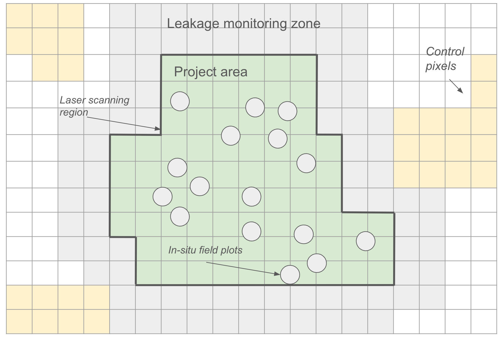
Figure 3. Schematic of the various monitoring locations referred to throughout this Protocol.
12.3
Project Area
The entire project area in Figure 1 must be monitored for the duration of the Project Commitment Period (see Section 5.1).
During the Crediting Period, monitored parameters from an AGB proxy map (e.g., canopy height) in the project area is used in conjunction with control pixels to establish a dynamic baseline for determining the additionality of carbon storage in the project area. It is highly recommended that Isometric or another independent third party be responsible for project area monitoring for establishing relative change compared to control pixels (see Section 12.4). Project Proponents may carry this monitoring out themselves provided that a transparent and reproducible monitoring plan is agreed upon ahead of time with Isometric.
After the Crediting Period, ongoing monitoring of forest biomass (e.g., forest cover or saturation index) must continue annually until the end of the Project Commitment Period for detection of Reversals (see Section 10.5). Isometric will ensure independent ongoing monitoring for Reversals until the end of the Project Commitment Period.
12.4
Control Pixels
Control pixels are used to assess natural regeneration in similar land areas outside the project area to determine the additional carbon storage of a reforestation project beyond the counterfactual scenario. Control pixels are selected by matching each project area pixel to a number of pixels outside the project area that historically behaved similarly (see Section 9.4.3).
An AGB proxy map (e.g., canopy height) is used to determine the relative difference in forest carbon between The Project and Counterfactual scenario for each Reporting Period (see Section 9.4). It is highly recommended that Isometric or another independent third party be responsible for selection and monitoring of control pixels. Project Proponents may carry this monitoring out themselves provided that a transparent and reproducible monitoring plan is agreed upon ahead of time with Isometric.
12.5
Leakage Monitoring Zone
For projects without sufficient activity-shifting leakage mitigation, the Leakage Monitoring Zone must be monitored using satellite imagery for the duration of the Crediting Period to detect deforestation near the project area. Annual monitoring of forest cover over time is used to calculate deforestation rates over time. See Section 8.3.6 for more details on how leakage monitoring is used.
It is highly recommended that Isometric or another independent third party be responsible for monitoring of the Leakage Monitoring Zone. Project Proponents may carry this monitoring out themselves provided that a transparent and reproducible monitoring plan is agreed upon ahead of time with Isometric, and will be checked annually by Isometric.
12.6
Laser Scanning Region
Airborne laser scanning measurements are only applicable for projects that wish to use regional LiDAR models to estimate AGB (Option 2 described in Section 9.3.2.2). ALS data collection should occur throughout the Crediting Period, at the end of each Reporting Period. Measurements should be taken in the same season (e.g., leaf-off) to reduce uncertainty and biases.
Wall-to-wall laser scanning measurements are highly recommended. Laser scanning of representative subplots throughout the project area is also permissible with rigorous statistical analysis to constrain the uncertainty associated with subplot selection and upscaling. See Section 9.3.2.2 and Appendix C for more information on laser scanning requirements.
12.7
In situ Field Plots
In situ field measurements are required for all projects throughout the Crediting Period. Field plots may be used as the primary method for calculating aboveground biomass (Option 1 in Section 9.3.2.1), or are used for benchmarking regional or global AGB maps (Option 2 in Section 9.3.2.2, or Option 3 in Section 9.3.2.3). For projects using Option 1, where AGB is derived directly from field measurements, then in situ field plots must be sampled at the beginning and end of each Reporting Period. Otherwise for Options 2 and 3, field measurements must be taken at a minimum of every 5 years for benchmarking AGB models.
See Appendix B for general guidance on field plot surveys, and Sections 9.3.2.1 - 9.3.2.3 for specific field plot requirements for each quantification approach. At minimum, species identification and DBH must be measured for all trees with DBH > 10 cm within the in situ field plot.
12.7.1
Monitoring before First Verification
During the first few years after planting seedlings, there may not be many trees with DBH > 10 cm. However, it is still important to monitor field plots during this time as young forests are particularly vulnerable to disease, ecological hazards, and may experience high rates of mortality. In addition, techniques to quantify forest biomass tend to overestimate in young forests. Between project initiation and first Verification (see Section 5), it is recommended to monitor for early tree mortality every 6 months to better constrain early stage growth as well as inform any mortality mitigation activities (e.g., replanting trees).
12.8
Summary of Monitoring Requirements
Table 2 Summary of the required and recommended monitoring parameters.
| Frequency | Location | Parameter | Methods | Justification | Recommended or Required | Responsible party |
|---|---|---|---|---|---|---|
From initial planting to first Verification, recommended every 6 months | In-situ field plots | Tree mortality | Mortality survey, or high resolution drone imagery | Estimations of forest biomass may be highly uncertain during the initial years after tree planting due to high rates of tree mortality and biases in young forests. Surveys for early tree mortality can better constrain early stage biomass growth, and enable mortality mitigation activities | Recommended | Project Proponent |
At the start and end of each Reporting Period for Option 1 in Section 9.3.2.1. Otherwise, at least every 5 years. | In situ field plots | DBH for all trees larger than 10 cm diameter | Tape measure | Fundamental measurement estimating AGB using allometric equations | Required | Project Proponent |
At the start and end of each Reporting Period for Option 1 in Section 9.3.2.1. Otherwise, at least every 5 years. | In situ field plots | Tree species | Ecologist identification | Necessary for selecting species-specific allometric equations and parameters | Required | Project Proponent |
At the start and end of each Reporting Period, e.g., once a year in the same season | Laser scanning plots | 3D Point clouds and derived metrics (e.g., canopy height) | Laser scanning instruments mounted on aerial | To derive estimates of forest aboveground biomass | Required for Option 2 (Section 9.3.2.2), otherwise not applicable | Project Proponent |
At the start and end of each Reporting Period, e.g., once a year in the same season | Project area | AGB Map | Satellite data or third-party mapped product | To derive estimates of forest aboveground biomass | Required for Option 3 (Section 9.3.2.3), otherwise not applicable | Isometric or a third party |
| At the start and end of each Reporting Period, e.g., once a year in the same season | Control pixels & project area | Forest carbon proxy (e.g, canopy height, biomass saturation index) | Satellite data or third-party mapped product | To quantify relative change in forest carbon sequestration between control pixels and project area (Equation 18) | Required | Isometric or a third party |
| At the start and end of each Reporting Period, e.g., once a year in the same season | Leakage buffer zone | Indicators of deforestation | Satellite | To identify any activity-shifting leakage that should be taken into account for the net carbon removal calculation (Equation 9) | Required | Isometric or a third party |
From the end of the Crediting Period to the end of the Project Commitment Period, annually | Project area | Indicators of deforestation | Satellite | To identify Reversals and appropriately remediate through the Buffer Pool | Required | Isometric or a third party |
13.0
Appendix A: Default Values for IS and NL Parameters
Isometric has carried out a literature review of and values to inform , as well as values for for certain regions. Where The Project falls into these regions, the default values provided must be used. This is because understanding which values to use from literature is challenging as academic papers are typically not written with this purpose or audience in mind. Isometric has completed this work for certain regions to lessen this complexity and provide consistency across projects.
These default values also serve as an example of appropriate values to select, however it should be noted that the quality of research differs across regions.
The following sections set out the procedure to be followed to obtain and values and set out the default values to be used for the regions studied.
13.1
Regions Studied
The regions considered in the literature review were:
- Brazil
- Panama
- Mexico
- United States
These regions were selected following a review of projected project demand. Isometric will update this analysis with additional regions iteratively based on demand. Values for other regions will be reviewed by Isometric on a case by case basis.
13.2
Values
IS represents the amount of production that is diverted to other locations. The IS value does not provide any information on where or in what manner that production is produced.
Procedure for determining values:
- Define a crop-region pair broadly enough to reasonably assume that the supply of all other crop and regions is zero. For example, for livestock, “beef in Mato Grasso” is too specific and “all meat globally” is too broad, “beef in South America” may come closer to a balance.
- Examine the existing academic literature for papers that estimate the supply/demand of the crop-region pair or some other similar pair. For example, we might use “meat in South America” in lieu of “beef in South America” if the former estimates are available.
- Ensure that the paper meets the criteria for a valid estimate:
- Analysis uses either a “dynamic panel” or “instrumental variables” technique.
- Based on time-series variation in prices, rather than cross-sectional (i.e., using prices that are varying over time, rather than spatial differences in transportation costs).
- Published in the last 15 years in a reputable economics or land use journal, or is published in a report for a reputable organization such as the European Union or California Air Resources Board.
- Analysis clearly notes whether the estimate is to be interpreted as a short-run or long-run estimate.
- Analysis uses planting season prices (rather than harvest season).
- Use the appropriate formula to calculate from the supply and demand elasticity
- In cases where no academic literature exists in the relevant context, select the most similar available default value (e.g., for cocoa, we might use the default value for coffee).
Where possible:
- Supply and demand elasticities used should be estimated within the same paper; and
- Paper should be cited by a reputable organization compiling a meta-analysis or parameterizing a partial equilibrium model for policy analysis (CARB, EU, FAO, etc.).
Table A1. default values.
| Geography | Crop | εdc | εsc | IS | Key citation |
|---|---|---|---|---|---|
| Global | Calories (rice, wheat, corn, soy) | -0.05 | 0.12 | 0.70 | Roberts and Schlenker (2013)43 |
| Global | Coffee | -0.305 | 0.285 | 0.48 | Akiyama and Varangis (1990)44 |
| Global | Cocoa | -0.075 | 0.075 | 0.50 | Askari and Cummings (1977)45, Behrman (1965)46 |
| South America | Livestock | -0.40 | 0.4 | 0.5 | Fragoso et al. (2011) 47 |
| North America | Livestock | -0.40 | 1.6 | 0.80 | Mintert et al. (2009)48, Jeong (2019)49 |
13.3
Values
Procedure for determining values:
In an ideal world, there would be estimates of the specific types of land use that were converted and their locations. However, this data is not available. Instead, the Project Proponent should focus on the most important elements of potential land use change from a carbon emissions perspective. NL values proposed aim to capture the net effect of a one unit removal of crop area on forestland conversion. These NL values will be smaller in magnitude than NL values that incorporate the possibility of conversion of grazing land or the conversion of lower-value crops to higher-value crops. Focusing on forests is more tractable and likely provides a large share of the relevant land use change emissions, since forest conversion is relatively permanent in a way that livestock to cropland conversion is not. In general, the NL values are more speculative than the IS values and often rely on assumptions about the yield-price elasticity that have not been empirically confirmed.
There are possible methodologies for obtaining values, which are set out here. Method B is in most cases the preferred approach. This is because the necessary conditions to implement Method A (limited trade/ disconnected markets and demand driven quantity increase) are rarely met in practice. Method A should only be used in special cases and justified appropriately. Both methods are set out below:
- Method A: In cases where a large increase in deforestation has accompanied a large increase in cropland, the ratio of land deforested for agriculture to total new agriculture is taken. Note, this procedure is only accurate for cases where (1) the deforestation followed a large demand-driven increase in production and (2) where the land is not well-connected to international markets. This approach is not reflected in the default values, as it is not an acceptable methodology for the majority of crop-regions.
- Method B: In most cases, such as the US, analyses of large changes in land use due to a policy shock is relied upon, and then the ratio of the percentage change in agricultural land to the percentage change in production is taken. This way of calculating NL is represented in the following definition:
(Equation A1)
Where:
- is Gross New Production From Extensification due to .
- is Change in regional average yield due to .
- is Total land area under study.
- is a 1-tonne reduction in supply, or a 1-unit price increase.
is variable under the assumption that changes to supply are predominantly channeled through price changes50.
By dividing the numerator and denominator, the above equation can be reformulated as:
(Equation A2)
Where:
- is the change in area due to .
- is the change in yield due to .
- is a 1-tonne reduction in supply, or a 1-unit price increase.
The following default values have been gathered using Method B.
Table A2. default values.
| Geography | Crop | NL | Key citation |
|---|---|---|---|
| Brazil | cropland | 0.61 | Pendrill et al (2019)51 |
| US | cropland | 0.28 | Lark et al (2022)52 |
| Mexico | cropland | N/A | Can use Brazil value |
| Panama | cropland | N/A | Can use Brazil value |
| Brazil | livestock | 0.83 | Bowman (2012)53 |
| US | livestock | 0.20 | Wu (2000)54 |
| Mexico | livestock | N/A | Can use Brazil value |
| Panama | livestock | N/A | Can use Brazil value |
| Global | Coffee | 0.60 | Report: “60% of land suitable for coffee is forested”55 |
| Global | Other specialty crops | N/A | See: global coffee value |
14.0
Appendix B: Guidance for Field Measurements
14.1
Field Plot Survey Guidance
Field plot surveys can be used as a primary approach for quantifying AGB, used for training regional area-based LiDAR models, or benchmarking and calibrating various AGB models. This Appendix summarizes some general guidance for field plot surveys, but specific requirements will depend on the intended usage of the field data. See Section 9.3.2 of the Protocol for specific requirements for particular usages.
Project Proponents should follow best practices guidelines. Recommended resources for guidance on field plot surveys include:
- USFS Measurement guidelines for forest sequestration56;
- Climate Action Reserve’s inventory manual57;
- RAINFOR protocol, which has guidance on establishing plots, tree measurements, and data recording58; and
- The Canadian Forest Service best practices guide, particularly Section 5, which has specific guidance on ground plot measurements for developing and validating predictive models from co-located ground measurements and airborne laser scanning data33.
14.1.1
Guidance for Plot Design
Field plots should be designed with the following considerations in mind:
- The number of field plots needed will vary based on the size of the project area, but at minimum should be greater than 30, as the Central Limit Theorem suggests that the mean values from a population ≥ 30 will yield a normal distribution.
- It is recommended to strive to meet the industry standard for a forest inventory, which is to have enough plots to obtain a confidence interval of +/- 10% of the mean at either 90 or 95% confidence.
- It is also advantageous to have plot centers fixed across time to ensure forest change is accurately captured.
- It is recommended that in project areas with diverse forest conditions, plots be stratified by forest type and structure57, 33.
- Field plots should be a minimum of 0.5 ha in area, in order to:
- Support a normalized distribution in AGB34; and
- Reduce the impact of edge decisions by field staff (e.g., inclusion of trees on border of plot).
- Plot measurements should also be temporally aligned to the greatest possible extent with map products derived from remote sensing.
14.1.2
Data Collection
Tree species should be recorded and the following should be measured:
- Tree diameter at 1.3 m above the ground (diameter at breast height, or DBH) for all trees in the field plot with a diameter greater than 10 cm;
- Tree height for a subset of trees (e.g., selected using a basal-area factor prism); and
- GPS coordinates, recommend collecting multiple location measurements at each point of interest, using mapping-grade receivers or higher (capable of achieving < 3 m accuracy, e.g., 500 measurements at a rate of 1 point per second).
The timing and frequency of field measurements depends on the usage of the measurements.
- If measurements are going to be paired with additional remote sensing measurements, such as LiDAR, then the field and remote sensing measurements should be temporally close (e.g., taken in the same year and season).
- At a minimum, it is recommended to take field measurement every five years.
15.0
Appendix C: Guidance for Airborne Laser Scanning Data Collection and Model Development
The following section outlines guidance for Airborne Laser Scanning (ALS) measurements, specifically for the purpose of training regional area-based models to estimate forest carbon from LiDAR measurements. ALS data can also be used to develop other types of models for forest carbon, such as through Individual Tree Crown modeling. Individual Tree Crown modeling is not in scope for this current Protocol version, but guidelines may be included in future iterations.
Project Proponents should follow established best practices in White et al., 2013: A best practices guide for generating forest inventory attributes from airborne laser scanning data using an area-based approach (Version 2.0) 33.
15.1
Plot Selection for Obtaining Training Data
Training regional area-based ALS models requires a large amount of overlapping LiDAR and field measurements from the region in which the model will be applied. It is important that the training data have a sufficient number of plots that are representative of the project area. Furthermore, the training data should encompass a variety of forest stand ages, so that the model can perform well for young and mature forests.
Specific recommendations for plot selection:
- Plot selection should be based on stratification into stands using meaningful forest characteristics, such as forest age, species, site index, slope, etc. Plots should then be randomly placed within those stands.
- It is recommended to use Structurally Guided Sampling to ensure that plots representative of the study area are included for training. In Structurally Guided Sampling, ALS metrics (e.g., height) are used as the source of data for stratification. See Goodbody et al., 202359 for more details on Structurally Guided Sampling.
- The placement of sample plots should account for spatial auto-correlation, e.g., by setting a minimum distance between plots of 100 m, or based on the decorrelation length.
15.2
Data Acquisition
Project Proponents are referred to White et al., 201333 for guidance on data acquisition parameters. Specific best practices recommendations include:
- Along-track and cross-track overlap should be at least 50% and ideally up to 80% and 60%, respectively.
- Scan angle should be ≤12 degrees, depending on forest canopy cover. Dense canopies should be observed using a smaller scan angle to ensure some pulses can reach the ground.
- Pulse density should beat minimum ≥2-4 points per meter (ppm), rising to 20 ppm, with the final constraint being sufficient ground sampling through the forest canopy to obtain a digital elevation model of 1 m resolution or greater.
- This typically requires a minimum average ground point sampling of 1 ppm sub-canopy. Thus, in a sparse or leaf-off forest, pulse densities closer to 2-4 ppm may be needed, while in a dense tropical forest those closer to 20 ppm may be needed. Larger densities provide a diminishing return of meaningful information and require increased data storage and processing capacity33. The USGS provides some base specifications for its own acquisitions, which are often used as the basis for LiDAR-based forest inventories in the United States. Quality-level 2 and better are often considered operational.
- For model-assisted design frameworks, a minimum of 25% coverage of the project area (after removing areas with scan-angles >12%) is recommended, and a simple systematic sampling design (i.e., flight lines) should be sufficient in most cases. In some instances flight lines may need to be drawn in such a way as to ensure the intersection with all strata. Overlap is not expected here.
15.3
LiDAR Data Processing
Data processing techniques must be sufficiently documented to permit replication, including quality control, filtering, and statistical analysis. The recommended quality control process differs between instruments. A typical LiDAR processing workflow consists of the following steps:
- Ground point classification
- Derivation of a digital terrain model
- Height normalization (i.e., flatten the point cloud)
- Noise removal (i.e., data errors, power lines, etc.)
- Derivation of forest structure metrics
- The lidRmetrics package implements a large number of these statistical features
- Typical metrics include:
- The percent of points above a given threshold
- The percentage of points in different brackets
- Kernel Density Estimation of point cloud heights
- Statistical indices that characterize vertical complexity
White et al. 201333 outlines best practices for LiDAR acquisition, planning, and development.
- LiDAR returns below 2 meters should be excluded from analysis, as these typically represent understory vegetation and can weaken the relationship between ALS-derived metrics and biomass densities.
- For model development, LiDAR data should be "clipped" to match the plot area boundaries. Statistical features can then be computed from this clipped data to develop the model. The lidR package documentation provides an example of this process.
It should be emphasized that this is different from conventional, moderate resolution remote sensing workflows where the plots are typically treated as a point and are spatially intersected with the rasterized feature layers. This approach yields poor performance with LiDAR data.
15.4
Statistical Modeling
LiDAR-based AGB maps have been developed with a variety of statistical models, including:
- Parametric modeling techniques, e.g., linear regression or variants such as linear mixed-effects models and non-linear mixed effects models. These models have many desirable properties when combined with a design-based sample of forest inventory plots. However, these models are restricted by assumptions (e.g., normality) and usually work best in homogeneous forest ecosystems (e.g., pine plantations).
- Regression trees, e.g., Random Forests or Gradient Boosting. These are the most common techniques used to construct AGB maps. Algorithms like Random Forests are robust to features displaying multicollinearity (most of the features computed using packages like lidrmetrics or FUSION are highly correlated) and can identify high-dimensional interactions among the predictor features. However, Random Forests are not capable of extrapolating beyond the bounds of the dataset, as the algorithms work via a recursive partitioning of the observed feature space during training. As such, when using tree-based models, it is important to ensure the plot data captures the full variability of the landscape. This again highlights the benefit of using a stratified or structurally guided sampling approach60.
- Deep learning, e.g., Neural Networks or Convolutional Neural Networks61. Deep learning methods are highly data depending and require a very large number of plot acquisitions. As such, it is common to pretrain these models on large datasets and then “tune” them on a local plot dataset.
It is recommended to use the simplest possible statistical model that yields high-performance on the modeling dataset.
Models used to estimate AGB should:
- Be based on peer-reviewed methodologies;
- Be applicable to the project area. See Meyer and Pebesma, 202162 and Johnson et al., 202263 for guidance on how to assess this; and
- Have a detailed workflow that justifies:
- Model selection (e.g., why was Random Forest chosen?)
- Model architecture (e.g., for deep learning, number of hidden layers)
- Dataset collation (e.g., where did it come from, how was data split for training/validation/testing)
- Model accuracy (e.g., AGB estimates and associated errors should be provided)
15.4.1
Notes on Additional Modeling Considerations
Non-parametric models commonly exhibit a phenomena called “regression-to-the-mean”. Machine learning models work by optimizing a loss function with the goal of obtaining the lowest possible error rate. Often, the lowest possible error will be obtained by over-estimating areas with low AGB densities and under-estimating areas with large AGB densities. This can be observed in the one-to-one regression plots of many papers (e.g., see Figure 3, Panel 1 in Pflugmacher et al., 2014)64.
When a model exhibits regression to the mean, it is not appropriate to simply sum the pixel values within a given area as the systematic error of the model has not been accounted for. This is a considerable problem for regrowth modeling. Non-parametric models that use satellite imagery will almost always dramatically over-estimate low-biomass densities. Similarly, there is good evidence that the “green-up” of stands to pre-disturbance levels in moderate resolution vegetation indices will predate the actual structural regeneration of the stand by many years65.
Model-assisted estimation is a framework that allows ancillary information to be incorporated into the estimation procedure. This can allow for more precise estimates of AGB density. The typical setup for a model-assisted estimation procedure is as follows:
- A design-based sample of the landscape has been acquired.
- A model (parametric or non-parametric) is then fit using ancillary datasets (e.g., multispectral features, LiDAR features, land cover information, etc.) and spatially applied to all pixels within the sampling domain.
- A model assisted estimator is then used that integrates the mapped predictions and the plots to produce a final estimate.
- It is worth noting that a model-assisted estimate of AGB will not be worse than a non-model assisted estimator. If the model that links the ancillary variables with the plot-level data is not performant, the model-assisted estimator will produce the same result as a non-model assisted estimator.
Details for model assisted estimation, and an associated R package, can be found in McConville et al., 2020 66.
Finally, it is worth nothing that there are many geostatistical considerations that come into play when developing statistical models. Spatial autocorrelation can violate the assumption of independence. This is why clustered plot designs are less efficient than other sampling schemes; the clustered plots are effectively pseudo-replicates. Under a design-based model-assisted framework, this is not a concern. However, it is a concern if the pixels in a map are being summed as all pixels within the same forest patch are pseudo replicates. Therefore, the sampling size is falsely inflated, given an optimistic estimate of the variance of the estimated mean.
16.0
Appendix D: Recommended Datasets and Resources
16.1
Allometry and Root-to-shoot Ratios
It is recommended to make use of root-to-shoot ratios that are developed in tandem with the allometry used. Allometric equations and root-to-shoot ratios should be selected based on the following hierarchy:
- Equations developed for national forest inventories
- IPCC generalized equations for different forest types
- Local peer-reviewed equations
For example in the United States, the National Scale Volume Biomass (NSVB) equations can be used, and these equations come with root allometry. The framework is explained in A national-scale tree volume, biomass, and carbon modeling system for the United States67 and the coefficients are given in the supplementary materials.
Furthermore, Allometric is an R package that curates allometric equations and facilitates their usage.
16.2
Land Cover Fraction
- Copernicus Global Land Cover Layers: CGLS-LC100 Collection 3 68 gives 100 m estimates of land cover fraction derived from Proba-V multispectral imagery and supplemental covariates.
- The ESA WorldCover 10 m is a discrete, and not fractional, product developed using Sentinel-1 radar and Sentinel-2 multispectral data69.
- Dynamic World is a 10 m, near-real time land use land cover layer produced by Google and distributed via Google Earth Engine. Note that this product is often best aggregated across a larger time-period for optimal accuracy70.
- Impact Observatory offers a free 10 m annual land cover layer based on Sentinel-2 multispectral data71.
17.0
Appendix E: Future Improvements
Additionality
- Currently, this Protocol uses a project-specific performance benchmark against control pixels to determine environmental additionality. Future versions of the Protocol may explore using remote sensing data to further create performance benchmarks to assess financial and regulatory additionality of The Project.
Approved Resources and Third-Party Datasets
- Isometric will develop and maintain a list of approved resources and third-party datasets for various parameters (e.g., carbon fractions, land cover classification maps, risk assessment) for different regions and biomes. Isometric will use this list for all relevant in-house monitoring processes, and Project Proponents must choose resources from this list unless they provide reasonable justification for a deviation (e.g., a new peer-reviewed publication that advances local knowledge).
Albedo
- Currently, albedo effects are not quantified since projects cannot be located in regions where albedo changes result in net warming. Incorporation of albedo impacts into this Protocol will be regularly reviewed.
Baseline
- Prior research on dynamic baselines have mostly been in the context of REDD+ and not reforestation. Pixel matching routines, statistical criteria and uncertainty will be revisited regularly to stay up to date with latest scientific developments.
Buffer Pool Contribution
- Isometric will review and adapt third-party tools and datasets, such as buffer pool density maps, as they become publicly available to enable project- and site-specific determination. Buffer Pools will be reassessed and scaled as appropriate to account for risk amplification or mitigation due to management activities and climate change.
Insurance
- Insurance providers can provide a third party risk assessment, are financially incentivized to correctly price risk, and have a fiduciary responsibility to pay out in the event of a Reversal. Presently, insurance cannot be used for the purpose of reducing Buffer Pool allocation size. This is due to limitations in the transparency in risk calculations, lack of data to substantiate risk models, and lack of supply of high quality Carbon Credits. As this area develops, insurance will be considered for inclusion in future versions of the Protocol. At minimum, insurance solutions must provide coverage for the entirety of the Project Commitment Period, either through a policy which extends for the full Project Commitment Period (e.g., 100 year policy) or an insurance contract extending for the full Project Commitment Period (e.g., 1 year policy with contract for 100 years).
Quantification with LiDAR
- Terrestrial laser scanning systems offer promise in quantifying forest biomass. Guidance on requirements and best practices for the use of terrestrial laser scanning and being considered for future versions of this Protocol.
- Individual tree crown (ITC) modeling is an alternative quantification approach. Detailed requirements for ITC modeling, LiDAR data used for ITC and allowable errors, will be considered for future versions of this Protocol.
Leakage
- Future versions may involve more reliance on leakage mitigation and eligibility requirements and possible removal of the leakage discounting.
- Currently, the Protocol assumes ecological leakage is zero. This will be revisited in future updates and included, where appropriate, in leakage assessment and leakage mitigation, especially in relation to areas sensitive to disease.
- Future versions of this Protocol may consider other land use activity-shifting leakages beyond deforestation.
- Future revisions of this Protocol will consider appropriate requirements for remote sensing data used for determining productivity.
Leakage Mitigation
- ‘Within project’ mitigation, such as timber harvesting and agroforestry, may be included in future modules.
Restoration Plan
- Further requirements around seedling to germplasm pipeline will be considered for future versions of the Protocol.
Stakeholder Engagement
- More detailed guidance on stakeholder identification and differentiation will be considered for future versions of the Protocol.
- Additional guidance on due diligence required to demonstrate that stakeholder rights are upheld will be considered for future versions of the Protocol.
Uncertainty
- Project Proponents are expected to quantify and justify the uncertainty associated with each parameter in the carbon removal calculation.
- Additional guidance on model validation metrics will be considered for future improvements.
- Isometric will consider providing a case study of uncertainty propagation for forest carbon stock quantification.
Project Deviations
- Isometric will develop procedures for changes to Crediting Projects such as project expansion or grouping.
Emergency Response
- Isometric may develop further guidelines on emergency response planning for disease, illegal logging, and forest fires.
18.0
Appendix F: Reforestation Risk Assessment
The Reforestation Risk Assessment is used to assess the overall delivery and storage risk associated with reforestation and may inform the Buffer Pool contribution during Credit delivery (see Section 10.4). The assessment must first be filled in by the Project Proponent and must be validated by a VVB. During project Validation, discrepancies between the Project Proponent’s self reported score and VVB may result in monitoring or risk mitigation activities, or project ineligibility. Eligible projects must have an initial risk score ≤ 20 and initial risk category scores at or below the following thresholds:
- Project Proponent Capacity Risk ≤ 7
- Financial Viability Risk ≤ 8
- Social Governance Risk ≤ 11
- Disturbance Risk ≤ 12
All risk categories shall have a minimum score of 0, regardless of the outcome of the Reforestation Risk Assessment.
If Project Proponents choose to forgo a flat 20% Buffer Pool contribution (see Section 10.4.1), the Reforestation Risk Assessment will inform Buffer Pool contributions for The Project according to the process outlined in Appendix G for each Reporting Period and in accordance with the requirements in Section 10.3.
- After each new Reforestation Risk Assessment evaluation, Isometric will update the required percentage of newly issued Credits that must be contributed to the Buffer Pool by The Project. We encourage Project Proponents to continuously monitor, mitigate, and reduce risks.
Table F1. Reforestation Risk Assessment, with the score to be filled out for each question.
| Risk Category | Risk Indicator | Evidence | Scoring Guidelines | Score |
|---|---|---|---|---|
| Project Proponent Capacity Risk | Does the Project Proponent maintain staff with domain expertise relevant for forest carbon projects? (e.g., forest ecology, forest measurement, carbon accounting) | Project’s team structure | If no, describe how gaps in relevant expertise will be filled, +1. | |
| Does the Project Proponent maintain a staff presence in the local vicinity (within one day of travel) of the project site? | Project’s team structure | If no, +2. | ||
| Was the Project Proponent established more than 12 months ago? | Project Proponent declaration | If no, +1. | ||
| Does the Project Proponent have prior experience in ecosystem restoration, carbon projects or planting? | Review of Project Proponent provided evidence and independent research | If yes, -1. | ||
| Has the Project Proponent abandoned or failed previous projects? | Review of projects on other registries | If yes, +3. | ||
| What proportion of the project area requires active enforcement against external threats (e.g., illegal logging, agricultural encroachment, unauthorized grazing) to protect carbon stocks? | Peer-reviewed publications, local or national government databases, NGO reports and assessments, site security assessment, satellite data, data on enforcement from other reforestation projects in the same region, local or national reports on environmental crimes or violations |
| ||
| Financial Viability Risk | Has The Project secured funding to cover all activities required before carbon revenue accrues? | Project financial plan |
| |
| What is the projected time to reach financial breakeven? | Project financial plan |
| ||
| Is the budget reasonable given the proposed project activities and ex-ante estimates for forest growth? Budget should at minimum include: personnel, equipment and supplies, infrastructure, travel and certification fees. | Project financial plan | If no, +2. | ||
| Does the project financial plan demonstrate sufficient cash flow throughout the Ongoing Monitoring Period to maintain forest carbon stocks? | Project financial plan | If continued financial incentive is low compared to likely opportunity cost of harvest, +2. | ||
| Does the project financial plan rely on future increases in market price for Carbon credits? | Project financial plan | If yes, +1. | ||
| Social Governance Risk | Are there currently or have there been disputes over land ownership over the last 20 years? | Jurisdictional history | If yes, +2. | |
| Does the government have a history of revoking legal agreements regarding land ownership, access, and usage? | Jurisdictional history | If yes, +2. | ||
| Does the project host country score below the 40th percentile on 3+ of the Worldwide Governance Indicators over the last 10 years? | Worldwide Governance Indicators | If yes, +2. | ||
| Does the government have an NDC in place that addresses corresponding adjustments/prevents double-counting of project Credits and NDC contributions? | National registries | If no, +1. | ||
| Does The Project have a detailed benefit-sharing plan that includes: clear distribution mechanisms, transparent criteria for beneficiary selection, a grievance resolution process, monitoring and reporting procedures? | Project financial plan |
| ||
| Does the Project Proponent have a presence on human rights, environmental or labor infraction lists? | National registries | If yes, fail. | ||
| Does the Project Proponent have ongoing legal disputes? | National registries | If yes, +1. | ||
| Does the Project Proponent have a presence in negative press content? | Online search | If yes, +1. | ||
| Have projects on Indigenous or Community Lands been identified? | Cross reference project documentation with Global Forest Watch | If no, fail. | ||
| Are baseline activities primarily subsistence-driven? | Land use documentation, Socioeconomic surveys |
| ||
| (a) Are there anticipated or demonstrated net positive community impacts? | Community impact assessment, project financial plan, socio-economic surveys | If no, +2. | ||
| (b) What is the net present value (NPV) of alternative land use compared to project NPV? | NPV analysis comparing alternative uses to project activities over Crediting Period, price forecasts, discount rate justification |
| ||
| Are opportunity cost risk mitigations in place? | Legal agreements protecting carbon stocks, Non-profit status documentation, grant/funding agreements |
| ||
| Disturbance Risk | Fire risk | Global Fire Weather Index |
| |
| Pest and disease outbreak risk | Regional third-party maps, if available. |
| ||
| Extreme weather (temperature - heat and cold) | IPCC AR6 24 |
| ||
| Extreme weather (hydrologic - flood and drought) | IPCC AR6 24 |
| ||
| Coastal risks (sea level rise, storm surge, tropical cyclones, salinity intrusion) | Regional third-party maps, if available. |
| ||
| Geologic risks (earthquakes, tsunami, volcanoes) | NOAA NCEI Natural Hazards viewer | If historical hazards in area, +1. | ||
| Illegal timber risk | Country IDAT risk score |
| ||
| Surrounding anthropogenic activities pose environmental risk (e.g., toxic pollution, industrial farming, new developments etc.) | Satellite imagery, site visit | If yes, +1. | ||
| Ecological Resilience | Project Design Document |
|
19.0
Appendix G: Buffer Pool Contributions
By default, projects are subject to a flat 20% Buffer Pool contribution as outlined in Section 10.4.1. Project Proponents may opt to calculate a project-specific Buffer Pool contribution based on the outputs of their Reforestation Risk Assessment for each Reporting Period.
The following steps are used to convert the outputs of the Reforestation Risk Assessment into a Buffer Pool contribution:
- Sum the total score for each risk category in Table F1.
- Map the risk score for each risk category into a Buffer Pool contribution using Table G1.
- Sum the Buffer Pool contribution for each risk category to obtain the total Buffer Pool contribution.
Table G1. Risk score to Buffer Pool contribution conversion for each risk category.
| Risk Category | Cumulative Risk Score | Buffer Pool Contribution |
|---|---|---|
| Project Proponent Capacity Risk | 0 | 2.5% |
| 1 | 3.3% | |
| 2 | 4.1% | |
| 3 | 5.5% | |
| 4 | 7.0% | |
| 5 | 8.4% | |
| 6 | 9.2% | |
| 7 | 10.0% | |
| Financial Viability Risk | 0 | 2.5% |
| 1 | 3.2% | |
| 2 | 3.9% | |
| 3 | 4.9% | |
| 4 | 6.2% | |
| 5 | 7.6% | |
| 6 | 8.6% | |
| 7 | 9.3% | |
| 8 | 10.0% | |
| Social Governance Risk | 0 | 2.5% |
| 1 | 3.1% | |
| 2 | 3.5% | |
| 3 | 4.0% | |
| 4 | 4.8% | |
| 5 | 5.7% | |
| 6 | 6.8% | |
| 7 | 7.7% | |
| 8 | 8.5% | |
| 9 | 9.0% | |
| 10 | 9.4% | |
| 11 | 10.0% | |
| Disturbance Risk | 0 | 2.5% |
| 1 | 3.1% | |
| 2 | 3.4% | |
| 3 | 3.9% | |
| 4 | 4.5% | |
| 5 | 5.3% | |
| 6 | 6.2% | |
| 7 | 7.2% | |
| 8 | 8.0% | |
| 9 | 8.6% | |
| 10 | 9.1% | |
| 11 | 9.4% | |
| 12 | 10.0% |
The Buffer Pool contribution for each risk category is determined using a sigmoid function described by Equation G1. The Buffer Pool contribution for each risk category ranges from 2.5% to 10%.
(Equation G1)
Where:
- is the Buffer Pool contribution for a given risk category.
- is the range of Buffer Pool contributions within each risk category (2.5% to 10%).
- is the steepness parameter of the sigmoid curve and determines how quickly the function transitions between its minimum and maximum values.
- is the midpoint of the sigmoid curve.
- is the risk score for a given risk category.
- is the value at which The Project fails the Reforestation Risk Assessment, noted in Appendix F.
The sigmoid function, Equation G1, applied to each risk category can also be visualized in Figure G1.

Figure G1. Buffer Pool contribution based on risk score for each risk category.
19.1
Project-Specific Buffer Pool Contribution Example
The Project has completed the Reforestation Risk Assessment and obtained the following risk scores in a Reporting Period:
- Project Proponent Capacity Risk = 2
- Financial Viability Risk = 4
- Social Governance Risk = 3
- Disturbance Risk = 3
Mapping these risk scores to Table G1, the total Buffer Pool contribution for The Project is:
4.1% + 6.2% + 4.0% + 3.9% = 18.2%
20.0
Acknowledgments
Isometric would like to thank following contributors to this Protocol:
- The Renoster team, particularly for contributions to the following sections: Quantification, Monitoring, guidance on field measurements and LiDAR measurements, Environmental and Social Safeguards
- Christopher Kilner, Ph.D. (Bird Conservancy of the Rockies)
- Matthew Gammans, Ph.D.
Isometric would like to thank following reviewers of this Protocol:
- Connor Nolan, Ph.D. (Stanford University)
- Anika Staccone, Ph.D.
- Ruben Dario Palacio, Ph.D. (Fundacion Ecotonos)
21.0
Definitions and Acronyms
- Above Ground Biomass (AGB)The total mass of living woody biomass existing above the soil surface in a specified area.
- ActivityThe steps of a Project Proponent’s Removal or Reduction process that result in carbon fluxes. The carbon flux associated with an activity is a component of the Project Proponent’s Protocol.
- AdditionalityAn evaluation of the likelihood that an intervention—for example, a CDR Project—causes a climate benefit above and beyond what would have happened in a no-intervention Baseline scenario.
- BaselineA set of data describing pre-intervention or control conditions to be used as a reference scenario for comparison.
- Below Ground Biomass (BGB)The total mass of living woody biomass existing below the soil surface in a specified area.
- BiodiversityThe diversity of life across taxonomic and spatial scales. Biodiversity can be measured within species (i.e. genetic diversity and variations in allele frequencies across populations), between species (i.e. the total number and abundance of species within and across defined regions), within ecosystems (i.e. the variation in functional diversity, such as guilds, life-history traits, and food-webs), and between ecosystems (variation in the services of abiotic and biotic communities across large, landscape-level scales) that support ecoregions and biomes.
- Buffer PoolA common and recognized insurance mechanism among Registries allowing Credits to be set aside (in this case by Isometric) to compensate for Reversals which may occur in the future.
- BuyerAn entity that purchases Removals or Reductions, often with the purpose of Retiring Credits to make a Removal or Reduction claim.
- Carbon Dioxide Equivalent Emissions (CO₂e)The amount of CO₂ emissions that would cause the same integrated radiative forcing or temperature change, over a given time horizon, as an emitted amount of GHG or a mixture of GHGs. One common metric of CO₂e is the 100-year Global Warming Potential.
- Carbon Dioxide Removal (CDR)Activities that remove carbon dioxide (CO₂) from the atmosphere and store it in products or geological, terrestrial, and oceanic Reservoirs. CDR includes the enhancement of biological or geochemical sinks and direct air capture (DAC) and storage, but excludes natural CO₂ uptake not directly caused by human intervention.
- Carbon FinanceResources provided to projects that are generating, or are expected to generate, greenhouse gas (GHG) Emission Reductions or Removals.
- CommodityA product that has been cultivated, raised or harvested primarily for food, shelter, or natural fiber.
- ConservativePurposefully erring on the side of caution under conditions of Uncertainty by choosing input parameter values that will result in a lower net CO₂ Removal or GHG Reduction than if using the median input values. This is done to increase the likelihood that a given Removal or Reduction calculation is an underestimation rather than an overestimation.
- CounterfactualAn assessment of what would have happened in the absence of a particular intervention – i.e., assuming the Baseline scenario.
- Cradle-to-GraveConsidering impacts at each stage of a product's life cycle, from the time natural resources are extracted from the ground and processed through each subsequent stage of manufacturing, transportation, product use, and ultimately, disposal.
- CreditA publicly visible uniquely identifiable Credit Certificate Issued by a Registry that gives the owner of the Credit the right to account for one net metric tonne of Verified CO₂e Removal or Reduction. In the case of this Standard, the net tonne of CO₂e Removal or Reduction comes from a Project Validated against a Certified Protocol.
- Crediting PeriodThe period of time over which a Project Design Document is valid, and over which Removals or Reductions may be Verified, resulting in Issued Credits.
- DeliveryThe outcome of a Project Proponent providing Credits to fulfill Buyers' purchases.
- Direct ActorA site owner, tenant or other user that engaged with the project site in a way that produced commodities before the project activities commenced.
- Direct EmissionsEmissions that are produced by a specific CDR process and are directly controllable.
- Double CountingImproperly allocating the same Removal or Reduction from a Project Proponent more than once to multiple Buyers.
- DurabilityThe amount of time carbon removed from the atmosphere by an intervention – for example, a CDR project – is expected to reside in a given Reservoir, taking into account both physical risks and socioeconomic constructs (such as contracts) to protect the Reservoir in question.
- Dynamic BaseliningA method for establishing and regularly updating the reference carbon stock levels in a reforestation project area, based on ongoing analysis of comparable non-project plots, to account for natural fluctuations and improve the accuracy of carbon credit calculations over the project lifetime.
- Ecological IntegrityThe ability of an ecosystem to support and maintain ecological processes and a diverse community of organisms. It is measured as the degree to which a diverse community of native organisms is maintained, and is used as a proxy for ecological resilience, intended as the capacity of an ecosystem to adapt in the face of stressors, while maintaining the functions of interest.
- Ecological ResilienceThe ability of an ecosystem to withstand and recover from disturbances while maintaining its structure and functions.
- Ecosystem FunctionThe natural processes and interactions that occur within an ecosystem, including the flow of energy and materials through biotic and abiotic components, encompassing activities like nutrient cycling, primary production, and habitat provision, which collectively maintain the balance and stability of the ecosystem.
- Embodied EmissionsLife cycle GHG emissions associated with production of materials, transportation, and construction or other processes for goods or buildings.
- Emission FactorAn estimate of the emissions intensity per unit of an activity.
- Emission ReductionsLowering future GHG releases from a specific entity.
- Environmental AdditionalityAn evaluation of the likelihood that an intervention causes a climate benefit above and beyond what would have happened in a no-intervention Baseline scenario.
- Ex-post CreditsIssuance of Credits after removal or reduction took place. This is the manner in which Isometric Delivers Credits.
- GHG StatementA document submitted alongside Claimed Removals and/or Reductions that details the calculations associated with a Removal or Reduction, including the Project's emissions, Removals, Reductions and Leakages, presented together in net metric tonnes of CO₂e per Removal or Reduction.
- Global Warming PotentialA measure of how much energy the emissions of 1 tonne of a GHG will absorb over a given period of time, relative to the emissions of 1 ton of CO₂.
- Greenhouse Gas (GHG)Those gaseous constituents of the atmosphere, both natural and anthropogenic (human-caused), that absorb and emit radiation at specific wavelengths within the spectrum of terrestrial radiation emitted by the Earth’s surface, by the atmosphere itself, and by clouds. This property causes the greenhouse effect, whereby heat is trapped in Earth’s atmosphere (CDR Primer, 2022).
- International Standards Organization (ISO)A worldwide federation (NGO) of national standards bodies from more than 160 countries, one from each member country.
- Invasive SpeciesA species whose introduction, spread, and/or growth threatens biological diversity.
- Issuance (of a Credit)Credits are issued to the Credit Account of a Project Proponent with whom Isometric has a Validated Protocol after an Order for Verification and Credit Issuance services from a Buyer and once a Verified Removal or Reduction has taken place.
- LeakageThe increase in GHG emissions outside the geographic or temporal boundary of a project that results from that project's activities.
- Leakage Mitigation SiteThe site(s) where leakage mitigation activities take place.
- Leakage Monitoring ZoneA transitional or boundary zone along the Project’s perimeter that is monitored for activity-shifting leakage.
- Light Detection and Ranging (LiDAR)LiDAR is a remote sensing technology that uses laser pulses to create highly accurate three-dimensional maps of forest structure, enabling measurements of tree height, canopy density, and biomass.
- Lossesfor open systems, biogeochemical and/or physical interactions which occur during the removal process that decrease the CO₂ removal .
- MaterialityAn acceptable difference between reported Removals/emissions or Reductions/emissions and what an auditor determines is the actual Removal/emissions or Reduction/emissions.
- ModelA calculation, series of calculations or simulations that use input variables in order to generate values for variables of interest that are not directly measured.
- ModuleIndependent components of Isometric Certified Protocols which are transferable between and applicable to different Protocols.
- Monitoring, Reporting, and Verification (MRV)The multi-step process to monitor the Removals or Reductions and impacts of a Project, report the findings to an accredited third party, and have this third party Verify the report so that the results can be Certified.
- PathwayA collection of Removal or Reduction processes that have mechanisms in common.
- ProjectAn activity or process or group of activities or processes that alter the condition of a Baseline and leads to Removals or Reductions.
- Project Design Document (PDD)The document that clearly outlines how a Project will generate rigorously quantifiable Additional high-quality Removals or Reductions.
- Project boundaryThe defined temporal and geographical boundary of a Project.
- ProtocolA document that describes how to quantitatively assess the net amount of CO₂ removed by a process. To Isometric, a Protocol is specific to a Project Proponent's process and comprised of Modules representing the Carbon Fluxes involved in the CDR process. A Protocol measures the full carbon impact of a process against the Baseline of it not occurring.
- ProxyA measurement which correlates with but is not a direct measurement of the variable of interest.
- RegistryA database that holds information on Verified Removals and Reductions based on Protocols. Registries Issue Credits, and track their ownership and Retirement.
- Remote SensingThe use of satellite, aircraft and terrestrial deployed sensors to detect and measure characteristics of the Earth's surface, as well as the spectral, spatial and temporal analysis of this data to estimate biomass and biomass change.
- RemovalThe term used to represent the CO₂ taken out of the atmosphere as a result of a CDR process.
- Reputable SourceA source that would be widely considered trustworthy based on the process undertaken (e.g., peer review) or origin of the information (e.g., government body).
- ReservoirA location where carbon is stored. This can be via physical barriers (such as geological formations) or through partitioning based on chemical or biological processes (such as mineralization or photosynthesis).
- ReversalThe escape of CO₂ to the atmosphere after it has been stored, and after a Credit has been Issued. A Reversal is classified as avoidable if a Project Proponent has influence or control over it and it likely could have been averted through application of reasonable risk mitigation measures. Any other Reversals will be classified as unavoidable.
- Sensitivity AnalysisAn analysis of how much different components in a Model contribute to the overall Uncertainty.
- SinkAny process, activity, or mechanism that removes a greenhouse gas, a precursor to a greenhouse gas, or an aerosol from the atmosphere.
- SourceAny process or activity that releases a greenhouse gas, an aerosol, or a precursor of a greenhouse gas into the atmosphere.
- StakeholderAny person or entity who can potentially affect or be affected by Isometric or an individual Project activity.
- StorageDescribes the addition of carbon dioxide removed from the atmosphere to a reservoir, which serves as its ultimate destination. This is also referred to as “sequestration”.
- System BoundaryGHG sources, sinks and reservoirs (SSRs) associated with the project boundary and included in the GHG Statement.
- UncertaintyA lack of knowledge of the exact amount of CO₂ removed by a particular process, Uncertainty may be quantified using probability distributions, confidence intervals, or variance estimates.
- Validation and Verification Bodies (VVBs)Third-party auditing organizations that are experts in their sector and used to determine if a project conforms to the rules, regulations, and standards set out by a governing body. A VVB must be approved by Isometric prior to conducting validation and verification.
Footnotes
-
van Diemen, R., Matthews, J. B. R., Möller, V., Fuglestvedt, J. S., Masson-Delmotte, V., Méndez, C., Reisinger, A., & Semenov, S. (Eds.). (2022). Annex I: Glossary. In P. R. Shukla, J. Skea, R. Slade, A. Al Khourdajie, R. van Diemen, D. McCollum, M. Pathak, S. Some, P. Vyas, R. Fradera, M. Belkacemi, A. Hasija, G. Lisboa, S. Luz, & J. Malley (Eds.), Climate Change 2022: Mitigation of Climate Change. Contribution of Working Group III to the Sixth Assessment Report of the Intergovernmental Panel on Climate Change. Cambridge University Press. https://doi.org/10.1017/9781009157926.020 ↩
-
Pan, Y., Birdsey, R. A., Fang, J., Houghton, R., Kauppi, P. E., Kurz, W. A., ... & Hayes, D. (2011). A large and persistent carbon sink in the world’s forests. Science, 333(6045), 988-993. https://doi.org/10.1126/science.1201609 ↩
-
Harris, N. L., Gibbs, D. A., Baccini, A., Birdsey, R. A., De Bruin, S., Farina, M., ... & Tyukavina, A. (2021). Global maps of twenty-first century forest carbon fluxes. Nature Climate Change, 11(3), 234-240. https://doi.org/10.1038/s41558-020-00976-6 ↩
-
Bastin, J. F., Finegold, Y., Garcia, C., Mollicone, D., Rezende, M., Routh, D., ... & Crowther, T. W. (2019). The global tree restoration potential. Science, 365(6448), 76-79. https://doi.org/10.1126/science.aax0848 ↩
-
Tierney, G. L., Faber-Langendoen, D., Mitchell, B. R., Shriver, W. G., & Gibbs, J. P. (2009). Monitoring and evaluating the ecological integrity of forest ecosystems. Frontiers in Ecology and the Environment, 7(6), 308-316. https://doi.org/10.1890/070176 ↩
-
FAO (2000). On Definitions of Forest and Forest Change. Forest Resources Assessment Programme, Working Paper 33, Rome. ↩
-
Hasler, N., Williams, C. A., Denney, V. C., Ellis, P. W., Shrestha, S., Terasaki Hart, D. E., ... & Cook-Patton, S. C. (2024). Accounting for albedo change to identify climate-positive tree cover restoration. Nature Communications, 15(1), 2275. https://doi.org/10.1038/s41467-024-46577-1 ↩
-
Dinerstein, E., Olson, D., Joshi, A., Vynne, C., Burgess, N. D., Wikramanayake, E., ... & Saleem, M. (2017). An ecoregion-based approach to protecting half the terrestrial realm. BioScience, 67(6), 534-545. https://doi.org/10.1093/biosci/bix014 ↩ ↩2
-
Besnard, S., Koirala, S., Santoro, M., Weber, U., Nelson, J., Gütter, J., ... & Carvalhais, N. (2021). Mapping global forest age from forest inventories, biomass and climate data. Earth System Science Data Discussions, 2021, 1-22. https://doi.org/10.5194/essd-13-4881-2021 ↩
-
Searle, E. B., & Chen, H. Y. (2017). Tree size thresholds produce biased estimates of forest biomass dynamics. Forest Ecology and Management, 400, 468-474. https://doi.org/10.1016/j.foreco.2017.06.042 ↩
-
Di Sacco, A., Hardwick, K. A., Blakesley, D., Brancalion, P. H., Breman, E., Cecilio Rebola, L., ... & Antonelli, A. (2021). Ten golden rules for reforestation to optimize carbon sequestration, biodiversity recovery and livelihood benefits. Global Change Biology, 27(7), 1328-1348. https://doi.org/10.1111/gcb.15498 ↩ ↩2 ↩3
-
Ewers, R. M., Orme, C. D. L., Pearse, W. D., Zulkifli, N., Yvon-Durocher, G., Yusah, K. M., ... & Banks-Leite, C. (2024). Thresholds for adding degraded tropical forest to the conservation estate. Nature, 631(8022), 808-813. https://doi.org/10.1038/s41586-024-07657-w ↩
-
Lindenmayer, D. B., & Luck, G. (2005). Synthesis: thresholds in conservation and management. Biological Conservation, 124(3), 351-354. https://doi.org/10.1016/j.biocon.2005.01.041 ↩
-
IUCN. 2024. The IUCN Red List of Threatened Species. Version 2024-1. https://www.iucnredlist.org. Accessed on [16 Oct. 2024]. ↩
-
Zhang, Y., Chen, H. Y., & Reich, P. B. (2012). Forest productivity increases with evenness, species richness and trait variation: a global meta‐analysis. Journal of ecology, 100(3), 742-749. https://doi.org/10.1111/j.1365-2745.2011.01944.x ↩
-
Pagad, S., Bisset, S., Genovesi, P., Groom, Q., Hirsch, T., Jetz, W., ... & McGeoch, M. A. (2022). Country compendium of the global register of introduced and invasive species. Scientific Data, 9(1), 391. https://doi.org/10.1038/s41597-022-01514-z ↩
-
van Kleunen, M., Pyšek, P., Dawson, W., Essl, F., Kreft, H., Pergl, J., ... & Winter, M. (2019). The global naturalized alien Flora (Glo NAF) database. ↩
-
Convention on Biological Diversity. (2002). Decision VI/23: Biodiversity and climate change. Retrieved from https://www.cbd.int/decision/cop/default.shtml?id=7197 ↩
-
Gann, G. D., McDonald, T., Walder, B., Aronson, J., Nelson, C. R., Jonson, J., ... & Dixon, K. (2019). International principles and standards for the practice of ecological restoration. Restoration ecology, 27(S1), S1-S46. https://doi.org/10.1111/rec.13035 ↩ ↩2
-
Höhl, M., Ahimbisibwe, V., Stanturf, J. A., Elsasser, P., Kleine, M., & Bolte, A. (2020). Forest landscape restoration—what generates failure and success?. Forests, 11(9), 938. https://doi.org/10.3390/f11090938 ↩ ↩2
-
United Nations General Assembly. (2007). United Nations declaration on the rights of indigenous peoples (A/RES/61/295). Retrieved from https://www.un.org/development/desa/indigenouspeoples/wp-content/uploads/sites/19/2018/11/UNDRIP_E_web.pdf ↩
-
United Nations. (2016). Free, prior, and informed consent: An indigenous peoples’ right and a good practice for local communities. Retrieved from https://www.un.org/development/desa/indigenouspeoples/publications/2016/10/free-prior-and-informed-consent-an-indigenous-peoples-right-and-a-good-practice-for-local-communities-fao/ ↩
-
Life cycle modules as described in BS EN 15978:2011 Sustainability of construction works — Assessment of environmental performance of buildings — Calculation method. https://knowledge.bsigroup.com/products/sustainability-of-construction-works-assessment-of-environmental-performance-of-buildings-calculation-method?version=standard ↩ ↩2 ↩3
-
IPCC, 2023: Climate Change 2023: Synthesis Report. Contribution of Working Groups I, II and III to the Sixth Assessment Report of the Intergovernmental Panel on Climate Change [Core Writing Team, H. Lee and J. Romero (eds.)]. IPCC, Geneva, Switzerland, pp. 35-115. https://doi.org/10.59327/IPCC/AR6-9789291691647 ↩ ↩2 ↩3
-
United States Energy Association (2022) Life Cycle Assessment of Carbon Dioxide Removal Methods Summary Report. Available at: https://usea.org/sites/default/files/USEA_CDR_LCA_SummaryReport_Final.pdf ↩
-
Cooper, J., Dubey, L., & Hawkes, A. (2022). Life cycle assessment of negative emission technologies for effectiveness in carbon sequestration. Procedia CIRP, 105, 357-361. https://doi.org/10.1016/j.procir.2022.02.059 ↩
-
Lefebvre et al. (2021) Assessing the carbon capture potential of a reforestation project. Available at: https://www.nature.com/articles/s41598-021-99395-6 ↩
-
IPCC (2003) Good Practice Guidance for Land Use, Land-Use Change and Forestry. Available at: https://www.ipcc.ch/site/assets/uploads/2018/03/GPG_LULUCF_FULLEN.pdf ↩
-
Doraisami, M., Kish, R., Paroshy, N. J., Domke, G. M., Thomas, S. C., & Martin, A. R. (2022). A global database of woody tissue carbon concentrations. Scientific Data, 9(1), 284. https://doi.org/10.1038/s41597-022-01396-1 ↩
-
Aalde, Harald. vol. 4, Nstitute for Global Environmental Strategies (IGES), 2006. IPCC Guidelines for National Greenhouse Gas Inventories: Agriculture, Forestry and Other Land Use. https://www.osti.gov/etdeweb/biblio/20880391 ↩ ↩2 ↩3
-
McGroddy, M. E., Daufresne, T., & Hedin, L. O. (2004). Scaling of C: N: P stoichiometry in forests worldwide: Implications of terrestrial redfield‐type ratios. Ecology, 85(9), 2390-2401. https://doi.org/10.1890/03-0351 ↩
-
Chave, J., Réjou‐Méchain, M., Búrquez, A., Chidumayo, E., Colgan, M. S., Delitti, W. B., ... & Vieilledent, G. (2014). Improved allometric models to estimate the aboveground biomass of tropical trees. Global change biology, 20(10), 3177-3190. https://doi.org/10.1111/gcb.12629 ↩
-
White, J. (2013). A best practices guide for generating forest inventory attributes from airborne laser scanning data using an area-based approach (INFORMATION REPORT FI-X-010). Natural Resources Canada. https://ostr-backend-prod.azurewebsites.net/server/api/core/bitstreams/3eac62d1-8765-48cb-a48e-a777eb8ae015/content ↩ ↩2 ↩3 ↩4 ↩5 ↩6 ↩7
-
Chave, J., Condit, R., Lao, S., Caspersen, J. P., Foster, R. B., & Hubbell, S. P. (2003). Spatial and temporal variation of biomass in a tropical forest: results from a large census plot in Panama. Journal of ecology, 91(2), 240-252. https://doi.org/10.1046/j.1365-2745.2003.00757.x ↩ ↩2
-
Ploton, P., Mortier, F., Réjou-Méchain, M., Barbier, N., Picard, N., Rossi, V., ... & Pélissier, R. (2020). Spatial validation reveals poor predictive performance of large-scale ecological mapping models. Nature communications, 11(1), 4540. https://doi.org/10.1038/s41467-020-18321-y ↩
-
Gao, S., Zhong, R., Yan, K., Ma, X., Chen, X., Pu, J., ... & Myneni, R. B. (2023). Evaluating the saturation effect of vegetation indices in forests using 3D radiative transfer simulations and satellite observations. Remote Sensing of Environment, 295, 113665. https://doi.org/10.1016/j.rse.2023.113665 ↩
-
An initial evaluation of carbon proxies for dynamic reforestation baselines. Pachama. Retrieved October 16, 2024, from https://pachama.com/blog/dynamic-reforestation-baselines/ ↩
-
Wilkinson, M. D., Dumontier, M., Aalbersberg, I. J., Appleton, G., Axton, M., Baak, A., ... & Mons, B. (2016). The FAIR Guiding Principles for scientific data management and stewardship. Scientific data, 3(1), 1-9. https://doi.org/10.1038/sdata.2016.18 ↩
-
Zolkos, S. G., Goetz, S. J., & Dubayah, R. (2013). A meta-analysis of terrestrial aboveground biomass estimation using lidar remote sensing. Remote sensing of environment, 128, 289-298. https://doi.org/10.1016/j.rse.2012.10.017 ↩ ↩2
-
Schwartzman, S., Lubowski, R. N., Pacala, S. W., Keohane, N. O., Kerr, S., Oppenheimer, M., & Hamburg, S. P. (2021). Environmental integrity of emissions reductions depends on scale and systemic changes, not sector of origin. Environ. Res. Lett, 16(9), 091001. https://doi.org/10.1088/1748-9326/ac18e8 ↩
-
Galik, C. S., Murray, B. C., Mitchell, S., & Cottle, P. (2016). Alternative approaches for addressing non-permanence in carbon projects: an application to afforestation and reforestation under the Clean Development Mechanism. Mitigation and adaptation strategies for global change, 21, 101-118. https://doi.org/10.1007/s11027-014-9573-4 ↩
-
Haya, B. K., Evans, S., Brown, L., Bukoski, J., Butsic, V., Cabiyo, B., ... & Sanchez, D. L. (2023). Comprehensive review of carbon quantification by improved forest management offset protocols. Frontiers in Forests and Global Change, 6, 958879. https://doi.org/10.3389/ffgc.2023.958879 ↩
-
Roberts, M. J., & Schlenker, W. (2013). Identifying supply and demand elasticities of agricultural commodities: Implications for the US ethanol mandate. American Economic Review, 103(6), 2265-2295. https://doi.org/10.1257/aer.103.6.2265 ↩
-
Akiyama, T., & Varangis, P. N. (1990). The impact of the International Coffee Agreement on producing countries. The World Bank Economic Review, 4(2), 157-173. https://doi.org/10.1093/wber/4.2.157 ↩
-
Askari, H., & Cummings, J. T. (1977). Estimating Agricultural Supply Response with the Nerlove Model: A Survey. International Economic Review, 18(2), 257. https://doi.org/10.2307/2525749 ↩
-
Jere Richard Behrman, 1965. "Cocoa: A Study of Demand Elasticities in the Five Leading Consuming Countries, 1950–1961," American Journal of Agricultural Economics, Agricultural and Applied Economics Association, 47(2), 410-417. https://ideas.repec.org/a/oup/ajagec/v47y1965i2p410-417..html ↩
-
Fragoso, R. M. D. S., Marques, C., Lucas, M. R., Martins, M. D. B., & Jorge, R. (2011). The economic effects of common agricultural policy on Mediterranean montado/dehesa ecosystem. Journal of Policy Modeling, 33(2), 311-327. https://doi.org/10.1016/j.jpolmod.2010.12.007. ↩
-
Mintert, J. R., Tonsor, G. T., & Schroeder, T. C. (2009). US beef demand drivers and enhancement opportunities: a research summary. https://beef.unl.edu/beefreports/symp-2009-14-xxi.shtml ↩
-
Jeong, S. (2019). The change in price elasticities in the US beef cattle industry and the impact of futures prices in estimating the price elasticities. Proceedings of the NCCC-134 Conference on Applied Commodity Price Analysis, Forecasting, and Market Risk Management. Minneapolis, MN. http://www.farmdoc.illinois.edu/nccc134 ↩
-
UN-REDD: Defintion of market leakage [Accessed October 2024]. Available at: https://www.un-redd.org/glossary/market-leakage#:~:text=Definition,actors%20to%20shift%20their%20activities ↩
-
Pendrill, F., Persson, U. M., Godar, J., & Kastner, T. (2019). Deforestation displaced: trade in forest-risk commodities and the prospects for a global forest transition. Environmental Research Letters, 14(5), 055003. https://doi.org/10.1088/1748-9326/ab0d41 ↩
-
Lark, T. J., Hendricks, N. P., Smith, A., Pates, N., Spawn-Lee, S. A., Bougie, M., Booth, E. G., Kucharik, C. J., & Gibbs, H. K. (2022). Environmental outcomes of the US Renewable Fuel Standard. Proceedings of the National Academy of Sciences, 119(9). https://doi.org/10.1073/pnas.2101084119 ↩
-
Bowman, M. S., Soares-Filho, B. S., Merry, F. D., Nepstad, D. C., Rodrigues, H., & Almeida, O. T. (2012). Persistence of cattle ranching in the Brazilian Amazon: A spatial analysis of the rationale for beef production. Land use policy, 29(3), 558-568. https://doi.org/10.1016/j.landusepol.2011.09.009. ↩
-
Wu, Z., Satter, L., & Sojo, R. (2000). Milk production, reproductive performance, and fecal excretion of phosphorus by dairy cows fed three amounts of phosphorus. Journal of Dairy Science, 83(5), 1028–1041. https://doi.org/10.3168/jds.s0022-0302(00)74967-8 ↩
-
Coffee Barometer. In Coffee Barometer (pp. 1–36). https://hivos.org/assets/2018/06/Coffee-Barometer-2018.pdf ↩
-
Pearson, T. R. (2007). Measurement guidelines for the sequestration of forest carbon (Vol. 18). US Department of Agriculture, Forest Service, Northern Research Station. https://doi.org/10.2737/NRS-GTR-18 ↩
-
Climate Action Reserve (2018). Standardized Inventory Methodlogy Version 1.0. https://www.climateactionreserve.org/wp-content/uploads/2018/06/Standardized-Inventory-Methodology_v1.0.pdf ↩ ↩2
-
Phillips, O., Baker, T., Feldpausch, T., & Brienen, R., (2001). RAINFOR Field Manual for Plot Establisment and Remeasurement. https://forestplots.net/upload/ManualsEnglish/RAINFOR_field_manual_EN.pdf ↩
-
Goodbody, T. R., Coops, N. C., Queinnec, M., White, J. C., Tompalski, P., Hudak, A. T., ... & Woods, M. E. (2023). sgsR: a structurally guided sampling toolbox for LiDAR-based forest inventories. Forestry, 96(4), 411-424. https://doi.org/10.1093/forestry/cpac055 ↩
-
Queinnec, M., Coops, N. C., White, J. C., McCartney, G., & Sinclair, I. (2022). Developing a forest inventory approach using airborne single photon lidar data: from ground plot selection to forest attribute prediction. Forestry: An International Journal of Forest Research, 95(3), 347-362. https://doi.org/10.1093/forestry/cpab051 ↩
-
Ayrey, E., Hayes, D. J., Kilbride, J. B., Fraver, S., Kershaw, J. A., Cook, B. D., & Weiskittel, A. R. (2021). Synthesizing disparate LiDAR and satellite datasets through deep learning to generate wall-to-wall regional inventories for the complex, mixed-species forests of the eastern United States. Remote Sensing, 13(24), 5113. https://doi.org/10.3390/rs13245113 ↩
-
Meyer, H., & Pebesma, E. (2021). Predicting into unknown space? Estimating the area of applicability of spatial prediction models. Methods in Ecology and Evolution, 12(9), 1620-1633. https://doi.org/10.1111/2041-210X.13650 ↩
-
Johnson, L. K., Mahoney, M. J., Bevilacqua, E., Stehman, S. V., Domke, G. M., & Beier, C. M. (2022). Fine-resolution landscape-scale biomass mapping using a spatiotemporal patchwork of LiDAR coverages. International Journal of Applied Earth Observation and Geoinformation, 114, 103059. https://doi.org/10.1016/j.jag.2022.103059 ↩
-
Pflugmacher, D., Cohen, W. B., Kennedy, R. E., & Yang, Z. (2014). Using Landsat-derived disturbance and recovery history and lidar to map forest biomass dynamics. Remote Sensing of Environment, 151, 124-137. https://doi.org/10.1016/j.rse.2013.05.033 ↩
-
Pickell, P. D., Hermosilla, T., Frazier, R. J., Coops, N. C., & Wulder, M. A. (2016). Forest recovery trends derived from Landsat time series for North American boreal forests. International Journal of Remote Sensing, 37(1), 138-149. https://doi.org/10.1080/2150704X.2015.1126375 ↩
-
McConville, K.S., Moisen, G. G., & Frescino, T. S. (2020). A Tutorial on Model-Assisted Estimation with Application to Forest Inventory. Forests. 11(2), 244. https://doi.org/10.3390/f11020244 ↩
-
Westfall, J. A., Coulston, J. W., Gray, A. N., Shaw, J. D., Radtke, P. J., Walker, D. M., Weiskittel, A. R., MacFarlane, D. W., Affleck, D. L., Zhao, D., Temesgen, H., Poudel, K. P., Frank, J. M., Prisley, S. P., Wang, Y., Meador, A. J. S., Auty, D., & Domke, G. M. (2023). A national-scale tree volume, biomass, and carbon modeling system for the United States. https://doi.org/10.2737/wo-gtr-104 ↩
-
Masiliūnas, D., Tsendbazar, N. E., Herold, M., Lesiv, M., Buchhorn, M., & Verbesselt, J. (2021). Global land characterisation using land cover fractions at 100 m resolution. Remote Sensing of Environment, 259, 112409. https://doi.org/10.1016/j.rse.2021.112409. ↩
-
Captain, N., Xu, P., Herold, M., Lesiv, M., Duerauer, M., Ruben Van De Kerchove, VITO, & Olivier Arino. (2022). Product Validation report. https://worldcover2021.esa.int/data/docs/WorldCover_PVR_V2.0.pdf ↩
-
Brown, C. F., Brumby, S. P., Guzder-Williams, B., Birch, T., Hyde, S. B., Mazzariello, J., Czerwinski, W., Pasquarella, V. J., Haertel, R., Ilyushchenko, S., Schwehr, K., Weisse, M., Stolle, F., Hanson, C., Guinan, O., Moore, R., & Tait, A. M. (2022). Dynamic World, Near real-time global 10 m land use land cover mapping. Scientific Data, 9(1). https://doi.org/10.1038/s41597-022-01307-4 ↩
-
Venter, Z. S., Barton, D. N., Chakraborty, T., Simensen, T., & Singh, G. (2022). Global 10 m land use land cover datasets: A comparison of dynamic world, world cover and esri land cover. Remote Sensing, 14(16), 4101. https://doi.org/10.3390/rs14164101 ↩
Contributors

Christopher Kilner, Ph.D.

Isometric

Jessica Hinojosa, Ph.D.

Stacy Kauk, P.Eng.

Jing He, Ph.D.

Emma Marsland

Marya Matlin-Wainer

Jennifer Yin, Ph.D.

Mark Allen
Changelog
Reforestation © 2025 Isometric HQ Ltd is licensed under CC BY-NC-ND 4.0