Contents
1.0
Introduction
This Protocol provides the requirements and procedures for the calculation of net carbon dioxide equivalent (CO2e) removal from the atmosphere via River Alkalinity Enhancement (RAE). This Protocol is developed for application in River Alkalinity Enhancement processes in which a cradle-to-grave GHG Statement can be accurately applied and in which the CO2 captured is durably stored for over 1000 years.
Rivers serve as the primary conduits of Earth’s terrestrial carbon cycle - connecting soils, the terrestrial biosphere and the atmosphere to the global ocean. Soils and shallow subsurface environments are the primary location of rock weathering, a process that releases alkalinity from carbonate and silicate minerals. Soil porewater, groundwater and their freshly weathered alkalinity are drained into rivers, where turbulent mixing allows for equilibration with the atmosphere and storage of CO2 in the form of dissolved inorganic carbon (DIC, predominately as bicarbonate and carbonate). Rivers then deliver some of this DIC to the global ocean, where it is durably stored for more than 10,000 years. Rivers are currently estimated to transport 0.3 - 0.5 GtC per year in the form of DIC to the global ocean, which currently stores approximately 40,000 GtC as DIC 1, ,2, 3, 4, 5. The addition of alkalinity to river systems for carbon dioxide removal takes advantage of these pre-existing natural processes that already transport and store significant amounts of carbon (Figure 1).

Figure 1 River alkalinity enhancement.
In rivers with favorable conditions, newly added alkaline feedstock will dissolve following the weathering reaction, leading to a net increase of carbon storage in the form of dissolved bicarbonate ions. For example, the dissolution of calcium carbonate (CaCO3) as an alkaline feedstock follows the chemical reaction:
Equation 1
Many rivers have chemical and physical characteristics that make them favorable for carbon removal via alkalinity enhancement. Compared to the ocean, rivers tend to have lower pH and are either undersaturated or kinetically inhibited with respect to carbonate mineral precipitation , thus favoring the dissolution of many potential alkaline feedstocks. Additionally, rivers are dynamic systems in which turbulent mixing allows newly-added alkalinity to equilibrate on relatively short timescales. The carbon stored as a result of RAE may come from direct drawdown from the atmosphere, or from dissolved CO2 sources (e.g., from microbial respiration, photo-oxidation of dissolved organic carbon, delivery of CO2-rich groundwater etc.) which would otherwise outgas to the atmosphere. The relative amount of each one of these carbon sources is determined by river characteristics such as discharge, local hydrology, incidence solar radiation, and other biogeochemical properties.
Although RAE for the purposes of carbon dioxide removal is relatively new, RAE has been conducted for decades as a remediation for pollution-related acid rain and river acidification. The introduction of alkaline feedstock, typically in the form of limestone, has been demonstrated as an effective tool for managing pollution-related river acidification and preserving habitat for some pH-sensitive species6, 7. These observations suggest that RAE at some locations may have additional ecological co-benefits.
This Protocol is developed to adhere to the requirements of ISO 14064-2: 2019 -- Greenhouse Gases -- Part 2: Specification with guidance at the project level for quantification, monitoring, and reporting of greenhouse gas emission reductions or removal enhancements. The Protocol ensures:
- Consistent, accurate procedures are used to measure and monitor all aspects of the RAE process required to enable accurate accounting of net CO₂e removals.
- Consistent system boundaries and calculations are utilized to quantify net CO₂e removal for RAE projects.
- Requirements are met to ensure the CO₂e removals are additional
- Evidence is provided and verified by independent third parties to support all net CO₂e removal claims.
Note that throughout this Protocol, use of the word "must" indicates a requirement, whereas "should" indicates a recommendation.
2.0
Sources and Reference Standards and Methodologies
Specific standards and protocols which are utilized as the foundation of this Protocol and for which this Protocol is intended to be fully compliant with are the following:
- Isometric Standard 1.0.0
- ISO (International Organization for Standardization) 14064-2: 2019 – Greenhouse Gases – Part 2: Specification with guidance at the project level for quantification, monitoring and reporting of greenhouse gas emission reductions or removal enhancements
Additional reference standards that inform the requirements and overall practices incorporated in this Protocol include:
- ISO 14064-3: 2019 - Greenhouse Gases - Part 3: Specification with Guidance for the verification and validation of greenhouse gas statements
- ISO 14040: 2006 - Environmental Management - Lifecycle Assessment - Principles & Framework
- ISO 14044: 2006 - Environmental Management - Lifecycle Assessment - Requirements & Guidelines
- A Code of Conduct for Marine Carbon Dioxide Removal Research, Aspen Institute, 2021
3.0
Future Versions
This Protocol was developed based on the current state of the art and current publicly available science regarding River Alkalinity Enhancement. As River Alkalinity Enhancement is a novel Carbon Dioxide Removal (CDR) approach, with limited published literature, the Protocol incorporates requirements that may be highly stringent to minimize risk and for the purposes of environmental and social safeguarding.
This Protocol will be altered in future versions as the science underlying this pathway evolves, and the overall body of knowledge and data across all processes is increased, for example regarding feedstock supply, weathering in river systems, ecological impacts and durable storage. Future updates will also increase the scope of eligible projects for this protocol.
This Protocol will be reviewed at a minimum every 2 years and/or when there is an update to scientific published literature which would affect net CO2e removal quantification or the monitoring and modeling guidelines outlined in this Protocol.
4.0
Applicability
The aim of this Protocol is to ensure that projects seeking carbon removal Credits for River Alkalinity Enhancement are safe and have a demonstrable net-negative climate impact. To be eligible for crediting under this Protocol, projects and associated operations must meet all of the following project conditions.
To ensure safety of human and environmental health, eligible projects must:
- Be officially permitted through relevant regulatory bodies.
- Characterize feedstock prior to usage according to the Rock and Mineral Feedstock Characterization Module v1.0, to ensure eligibility of feedstock selection and ecological suitability.
- Identify and take action to mitigate environmental and socio-economic risks, as described in Section 3.7 of the Isometric Standard and Section 6 of this Protocol.
To ensure net-negative climate impacts, eligible projects must:
- Be considered additional, in accordance with the requirements of Section 5.4.
- Provide a net-negative CO2e impact (net CO2e removal) as calculated in compliance with Section 8, on a cradle to grave GHG assessment basis.
- Provide long duration storage (>1,000 yr) of CO2 in seawater.
The following applicability requirements are to limit the scope of eligible projects that V1 of this protocol is developed for. However, these may be expanded in future iterations of the protocol.
- This Protocol currently includes storage of removed CO2 as Dissolved Inorganic Carbon (DIC) in the Ocean, thus only DIC that is exported from the river to the ocean is eligible for crediting. Long term storage in inland waters (e.g. lakes) will be explored for future Protocol iterations.
- This Protocol employs a simplified model and assumptions for river transport and biogeochemistry to quantify CO2 removal. To ensure responsible application of this Protocol, eligible Projects must meet the following criteria:
- The river transit time from dosing location to the river mouth must be under 1 week.
- There must be no hydraulic features which increase the mean transit time by 1 day between the dosing location and river mouth.
- The river must not discharge into salt marsh or mangrove dominated estuaries.
- The river’s downstream floodplain for 1-year flood must not be >20% of the river width.
- Dosing at locations with downstream wastewater treatment facilities discharging directly into rivers is not applicable. These sites may be eligible with additional monitoring upstream and downstream of the wastewater discharge site, and appropriate adaptations to the quantification framework.
This Protocol only quantifies CDR which results in pre-equilibrated alkalinity being transported to oceans as DIC via the river drainage network. Additional uptake of CO2 that occurs in the open ocean is not eligible for crediting under this Protocol.
5.0
Relation to the Isometric Standard
The following topics are covered briefly in this Protocol due to their inclusion in the Isometric Standard, which governs all Isometric protocols. See in-text references to the Isometric Standard for further guidance.
5.1
Project Design Document
For each specific project to be evaluated under this Protocol, Project Proponents must document project characteristics in a Project Design Document (PDD) as outlined in Section 3.2 of the Isometric Standard. The PDD will form the basis for project verification and evaluation in accordance with this Protocol, and must include consideration of processes unique to River Alkalinity Enhancement projects, such as:
- detailed feedstock characterization following the Rock and Mineral Feedstock Characterization Module v1.0;
- description of site and business as usual operations, following Section 10;
- description of the mitigation plan according to the environmental and social risk assessment in adherence with Section 6, including an accompanying robust monitoring plan to ensure efficacy;
- description of the quantification strategy for net CO2e removal following Section 8;
- description of all measurement and methods used to quantify processes relevant to the calculation of net CO2e removal, cross-referenced with relevant standards where applicable.
5.2
Verification and Validation
Projects must be validated and net CO2e removals verified by an independent third party, consistent with the requirements described in this Protocol as well as in Section 4 of the Isometric Standard.
The Validation and Verification Body (VVBs) must consider the following requisite components:
- Validate that the feedstock adheres to the requirements listed in the Mineral and Rock Feedstock Characterization Module v1.0.
- Verify that the quantification approach adheres to requirements of Section 8, including demonstration of required records.
- Verify that the Environmental & Social Safeguards outlined in Section 6 are met.
- Verify that The Project is compliant with requirements outlined in the Isometric Standard.
5.2.1
Verification Materiality
The threshold for Materiality, considering the totality of all omissions, errors and mis-statements, is 5%, in accordance with Section 4.3 of the Isometric Standard.
Verifiers should also verify the documentation of uncertainty of the GHG statement as required by Section 2.5.7 of the Isometric Standard. Qualitative Materiality issues may also be identified and documented, such as:
- control issues that erode the verifier’s confidence in the reported data;
- poorly managed documented information;
- difficulty in locating requested information;
- noncompliance with regulations indirectly related to GHG emissions, removals or storage.
5.2.2
Site Visits
Project validation and verification must incorporate site visits to project facilities in accordance with the requirements of ISO 14064-3, 6.1.4.2, including, at a minimum, site visits during validation and initial verification. Validators should, whenever possible, observe project operations to ensure full documentation of process inputs and outputs through visual observation (see Section 4 of the Isometric Standard).
A site visit must occur at least once per project validation.
5.2.3
Verifier Qualifications & Requirements
Verifiers and validators must comply with the requirements defined in Section 4 of the Isometric Standard. In addition, VVB teams shall maintain and demonstrate expertise associated with the specific technologies of interest, including fluvial modeling and measurement, analysis and data processing.
All VVBs are approved by Isometric independently and impartially based on alignment with Conflict of Interest policies, rotation of VVB policies, oversight on quality and the following requirements:
- VVBs must be able to demonstrate accreditation from:
- Alternatively, on a case-by-case basis, if VVBs are able to demonstrate to Isometric that they satisfy all required Verification needs and competencies required for the relevant Protocol and follow the guidelines of ISO 19011 or other relevant standards, they may be approved.
5.3
Ownership
CDR via River Alkalinity Enhancement can often be a result of a multi-step process (such as quarrying, alkaline feedstock processing, transportation, on-site operations and monitoring), with activities in each step managed and operated by a different operator, company or owner. When there are multiple parties involved in the process, and to avoid double counting of net CO₂e removal, a single Project Proponent must be specified contractually as the sole owner of Credits. Contracts must comply with all requirements defined in Section 3.1 of the Isometric Standard.
5.4
Additionality
The Project Proponent must be able to demonstrate additionality through compliance with Section 2.5.3 of the Isometric Standard. The counterfactual scenarios and baselines utilized to assess additionality must be project-specific, and are described in Section 8 of this Protocol.
Additionality determinations must be reviewed and completed every two years, at a minimum, or whenever project operating conditions change significantly, such as the following:
- regulatory requirements or other legal obligations for project implementation change or new requirements are implemented;
- project financials indicate Carbon Finance is no longer required, potentially due to, for example:
- increased tipping fees for waste feedstocks;
- sale of co-products that make the business viable without Carbon Finance;
- reduced rates for capital access.
Any review and change in the determination of additionality will not affect the availability of Carbon Finance and Credits for the current or past Crediting Periods, but, if the review indicates the project has become non-additional, this will make The Project ineligible for future Credits.
5.5
Uncertainty
The uncertainty in the overall estimate of net CO2e removal as a result of The Project must be accounted for. The total net CO2e removal for a specific Reporting Period must be conservatively determined, and projects must conduct an uncertainty analysis for the net CO₂e removal calculation in compliance with requirements outlined in Section 2.5.7 of the Isometric Standard.
5.5.1
Reporting of Uncertainty
Projects must report a list of all key variables used in the net CO2e removal calculation and their uncertainties, as well as a description of the uncertainty analysis approach, including:
- required measurements used for net CO2e removal calculation;
- emission factors utilized, as published in public and other databases used;
- values of measured parameters from process instrumentation, such as electricity usage from utility power meters;
- laboratory analyses, including analysis of seawater chemistry and alkaline feedstocks.
The uncertainty information should at least include the minimum and maximum values of each variable that goes into the net CO2e removal calculation (see Section 8 for more details). More detailed uncertainty information should be provided if available, as outlined in Section 2.5.7 of the Isometric Standard.
In addition, a sensitivity analysis that demonstrates the impact of each input parameter’s uncertainty on the final CO2e removal uncertainty must be provided. Details of the sensitivity analysis method must be provided such that a third party can reproduce the results. Input variables may be omitted from an uncertainty analysis if they contribute to a < 1% change in the net CO2e removal. For all other parameters, information about uncertainty must be specified.
5.6
Data Reporting and Availability
In accordance with the Isometric Standard, all evidence and data related to the underlying quantification of net CO2e removal and environmental monitoring will be available to the public through Isometric’s Science Platform. That includes:
- Project Design Document
- GHG Statement
- Measurements taken
- Model specifications and output
- Emission factors used
- Scientific literature used
The Project Proponent can request certain information to be restricted (only available to authorized buyers, the Registry and VVB) where it is subject to confidentiality. However, that does not apply to any numerical data produced or used as part of the quantification of net CO2e removal.
6.1
Overarching Principles
Following the Isometric Standard, Credits issued under this Protocol are contingent on the implementation, transparent reporting and independent verification of comprehensive safeguards. These safeguards encompass a wide range of considerations, including environmental protection, social equity, community engagement and respect for cultural values. The process mandates that safeguard plans be incorporated into all major project phases, with detailed reports made accessible to stakeholders. Adherence to and verification of environmental and social safeguards is a condition for all Crediting Projects.
6.2
Governance and Legal Framework
Projects must adhere to the following governance and legal requirements:
Official permitting:
- Project Proponents must identify jurisdictional authorities of water bodies of the project site, and as outlined in Section 4.
- Projects must receive official permitting and operate within the permitted discharge limits.
Compliance:
- Project Proponents must comply with all national and local laws, regulations and policies.
- Where relevant, projects must comply with international conventions and standards governing human rights and uses of the environment, when conducted within or foreseeably impacting Party jurisdictions.
6.3
Risk Mitigation Strategies
Environmental and social risk assessment in adherence with Section 3.7 of the Isometric Standard must be completed to identify potential risks, followed by the development of tailored mitigation plans. These plans must encompass specific actions to avoid, minimize or rectify identified impacts. Effective implementation of these measures must also be accompanied by a robust monitoring plan to detect negative impacts and stop projects when necessary (see Section 11).
Environmental and social risk identification, assessment, avoidance and mitigation planning will be unique to each Project’s technological, environmental and social contexts. The severity of these risks vary based on site specificities and the intensity and duration of alkalinity enhancement.
6.3.1
Environmental Safeguards
The Project Proponent must conduct an environmental impact assessment which adheres to Section 3.7.1 of the Isometric Standard.
When assessing aquatic environmental risks, it is important to holistically consider the risk compared to the baseline scenario. While the application of RAE for carbon dioxide removal is relatively new, river liming has been employed since the 1970s as a remediation tool to mitigate the influence of pollution-derived acid deposition on rivers. Given this relatively long history, the potential benefits and challenges associated with river liming are generally well understood6.
The application of alkaline feedstock to rivers can restore natural ecosystems and protect habitat and animal populations that are impacted by pollution-related pH changes. It can also lead to algal blooms and the introduction of harmful metals, either from feedstock dissolution or through the destabilization of sediment-hosted metals. Establishing a stable chemistry in the river by minimizing project-induced fluctuations in water quality is also important for maintaining overall river health. All of these factors need to be carefully considered when selecting a project location, feedstock, dosing rate, and other project specifications. Planning alkalinity dosing shcemes that sufficiently protect the riverine and downstream environment during project ramp-up and steady state operation is a pre-deployment requirement (see Section 10 for more details).
Ongoing monitoring for ecosystem safety (Section 11.4) is required to assess impacts due to subtle yet chronic changes to the environment. This includes reassessing if deployments are successful in their holistic goals of CDR and ecosystem restoration. The ecosystem monitoring needs may differ depending on the specific ecology of the site (such as microbial community structure, organic matter respiration, metals and nutrient budgets, etc.). These site-specific risks require input from subject matter and local expertise to devise responsible plans to address and mitigate unintended consequences. The monitoring plan for ecosystem safety must include sensitive zones along the river, which may include the weathering zone, estuary and ecologically important regions such as nurseries.
Particular environmental risks associated with River Alkalinity Enhancement which must be assessed, avoided and/or mitigated are:
Feedstock sourcing:
- Potential risks associated with feedstocks include land use impacts from sourcing, production, preparation, storage and distribution, such as land degradation, land occupation, dust pollution, deforestation and localized watershed contamination.
Co-products and waste:
- Generation of waste products or additional waste must be accompanied by a plan which ensures safe handling, containment and disposal.
Pollution prevention:
- Additional pollutants, such as nutrients or toxic elements, from dissolution of feedstock(s), which may result in bioaccumulation in biota or water quality impacts for downstream water users. Rock and Mineral Feedstock characterization is mandatory as a first line of defense for safeguarding against the release of harmful pollutants.
- Increased turbidity from feedstock addition or production of clays (in the case of aluminosilicate mineral feedstocks).
- Increased erosion and sediment delivery to the river during site construction.
- Accumulation of feedstock on the river bed may alter the sediment-water interface and impact benthic invertebrates.
- Removal of inorganic nutrients due to secondary mineral formation could drive nutrient limitation, resulting in a decrease in biological productivity or shift in ecosystem composition 8.
Ecological impacts:
- Shock to the ecosystem due to rapid or sudden changes in carbonate system parameters.
- Changes in carbonate chemistry, such as pH, could directly help or harm aquatic life depending on the magnitude and direction of the pH shift.
- Cascading impacts of altered carbonate chemistry, nutrient fields or particle deposition on biodiversity and ecosystem functions at and downstream of the water body.
- Site establishment may result in disturbances in the riparian zone.
6.4
Stakeholder Engagement
Per Section 3.5 of the Isometric Standard, Project Proponents must demonstrate active stakeholder engagement throughout project planning and operation, ensuring that all risk mitigation strategies contribute to sustainable project outcomes. Local stakeholders situated in the vicinity of the project site may contribute an in-depth understanding of the local system and provide invaluable insights and recommendations on the potential risks, necessary safeguards and specific monitoring needs. Relevant local stakeholders may include municipal utilities operators, local members of academia, Indigenous groups, environmental groups, and citizen associations. The Stakeholder Input Process must adhere to requirements outlined in Section 3.5 of the Isometric Standard, and evidence of these meetings must be submitted in the PDD.
6.5
Adaptive Management
Project Proponents must include in the PDD a plan for information sharing, emergency response and conditions for stopping or pausing alkaline feedstock dosing. Adaptive management plans must be in place in instances where:
- instrument malfunctions lead to data-gaps in required monitoring;
- dosing exceeds thresholds outlined in the PDD;
- regulatory non-compliance, e.g. danger to ecosystem health, is detected (such as by the local community or government agency);
- compromised health and/or safety of workers and/or local stakeholders.
The adaptive management plan must be designed to address and respond effectively to the needs of ecosystem and public health and safety. For instance, to mitigate potential shock to ecosystems, a reduction in alkaline feedstock dosing may be considered a more suitable approach than the complete cessation of dosing.
7.0
System Boundary and Baseline
7.1
Reporting Period
The Reporting Period represents an interval of time over which removals are calculated and reported for verification. The total net CO₂e removal is calculated using a series of measurements for a specified Reporting Period, and is written hereafter as .
GHG emission calculations must include all emissions related to the project activities that occur within the Reporting Period. This includes:
- any emissions associated with project establishment allocated to the Reporting Period,
- any emissions that occur within the Reporting Period,
- any anticipated emissions that would occur after the Reporting Period that have been allocated to the Reporting Period, and
- leakage emissions that occur outside of the system boundary as a result of induced market changes that are associated with the Reporting Period.
7.2
System Boundary & GHG Emissions Scope
The scope of this Protocol includes GHG sources, sinks and reservoirs (SSRs) associated with a River Alkalinity Enhancement (RAE) Project. A cradle-to-grave GHG Statement must be prepared encompassing the GHG emissions relating to the activities outlined within the system boundary. The system boundary must include all SSRs controlled by and related to The Project, including but not limited to the SSRs in Figure 2 and Table 1.
As noted in Section 7.3, the baseline scenario assumes river conditions in the absence of any River Alkalinity Enhancement project.

Figure 2 System boundaries for a River Alkalinity Enhancement (RAE) project.
The system boundary must include all GHG SSRs from activities related to the batch of Credits delivered within the Reporting Period that are associated with the establishment of The Project, operations and end-of-life activities that occur after the Reporting Period.
Any emissions from sub-processes or process changes that would not have taken place without the involvement of the CDR process, such as subsequent transportation, must be fully considered in the system boundary. This allows for accurate consideration of additional, incremental emissions induced by the CDR process.
If any GHG SSRs within Table 1 are deemed not appropriate to include in the system boundary, they may be excluded if robust justification and appropriate evidence is provided.
Table 1. Scope of activities and GHG SSRs to be included by the removal project
| Activity | GHG source, sink or reservoir | GHG | Scope | Timescale |
|---|---|---|---|---|
| Project Establishment | Initial surveys and feasibility studies | All GHGs | Any embodied, energy and transport emissions associated with surveys or feasibility studies required for establishment of the project site. | Before dosing starts - must be accounted for in the first Reporting Period or amortized in line with allocation rules (See Section 8.5.1) |
| Equipment and materials | All GHGs | Embodied emissions associated with equipment and materials manufacture related to project establishment (lifecycle modules A1-39). This must include product manufacture emissions for: Equipment (e.g., vehicles or machinery) Buildings/ structures (e.g., doser) Infrastructure (e.g., roads or footpaths) Temporary structures (e.g., fencing) | ||
| Equipment and materials transport to site | All GHGs | Transport emissions associated with transporting materials and equipment to the project site(s) (lifecycle module A49). | ||
| Construction and installation activities | All GHGs | Emissions associated with construction and installation of the project site(s) (lifecycle module A59) for RAE CDR activities and any additional infrastructure requirements as a result of RAE activities. To include energy use for construction, installation and groundworks, as well as waste processing activities and emissions associated with land use change. | ||
| Staff travel | All GHGs | Flight, car, train or other travel required for the project establishment, including contractors and suppliers required on site. | ||
| Misc. | All GHGs | Any SSRs not captured by categories above. | ||
| Operations | Energy use | All GHGs | Electricity and fuel consumption associated operational processes, including operation of dosing equipment, marginal pumping, pre-treatment, and discharge to the riverine environment. | Over each Reporting Period - must be accounted for in the relevant Reporting Period (See Section 8.5.2) |
| Feedstock manufacturing and transport | All GHGs | Feedstock raw material extraction and manufacturing including rock quarrying, crushing, grinding and drying. Feedstock transport from source manufacturer to project site. | ||
| Feedstock characterization | All GHGs | Embodied, energy use and transport emissions associated with sampling the feedstock to measure the physical and geochemical characteristics. | ||
| Consumables (other than feedstock) | All GHGs | Embodied emissions associated with consumables required for operation of the project site (excluding feedstock). This could include consumables for dosing equipment and other essential operations for CDR activities. | ||
| Maintenance of project site | All GHGs | To include maintenance (lifecycle modules B29), repair (B3), replacement (B4) and refurbishment (B5) activities associated with equipment, buildings and infrastructure. | ||
| Transport of dosing equipment | All GHGs | Transportation emissions for transport of dosing equipment around the site, if applicable. | ||
| Sampling required for MRV | All GHGs | Monitoring, including consumables used for measurement and transportation or shipping of samples for laboratory analysis and sample processing. | ||
| Staff travel | All GHGs | Flight, car, train, boat or other travel required for the project operations, including contractors and suppliers required on site. | ||
| Surveys | All GHGs | Embodied, energy and transport emissions associated with undertaking required surveys e.g. environmental impact surveys. | ||
| CO₂ stored | CO₂ | The gross amount of CO₂ removed and durably stored from the River Alkalinity Enhancement process as ocean dissolved inorganic carbon (DIC). | ||
| Misc. | All GHGs | Any SSRs not captured by categories above. For example, accidental or unintended release of treated waters may result in secondary precipitation and ocean outgassing, or unneutralized streams may result in ocean outgassing. If these events occur, their impacts must be quantified. | ||
| End-of-Life | End-of-life of project facilities and equipment | All GHGs | To include anticipated end-of-life emissions for project facilities and equipment, for example decommissioning of the dosing equipment (lifecycle modules C1-49). | After Reporting Period - must be accounted for in the first Reporting Period or amortized in line with allocation rules (See Section 8.5.3) |
| Ongoing surveys | All GHGs | Embodied, energy and transport emissions associated with undertaking long-term required surveys e.g. ecological surveys. | ||
| Misc. | All GHGs | Any emissions source, sink or reservoir not captured by categories above. |
The Project Proponent must consider all GHGs associated with SSRs, in alignment with the United States Environmental Protection Agency’s definition of GHGs, which includes: carbon dioxide (CO₂), methane (CH4), nitrous oxide (N₂O) and fluorinated gasses such as hydrofluorocarbons (HFCs), perfluorocarbons (PFCs), sulfur hexafluoride (SF6) and nitrogen trifluoride (NF3). For CO₂ capture and CO₂ leakage, only CO₂ is expected to be included as part of the quantification. For all other activities, all GHGs must be considered. For example, CO₂, CH4 and N₂O are all associated with diesel consumption.
All GHGs must be quantified and converted to CO₂e. GHGs must be converted to CO₂e in the GHG Statement using the 100-yr Global Warming Potential (GWP) for the GHG of interest, based on the most recent volume of the IPCC Assessment Report (currently the Sixth Assessment Report) 10.
Miscellaneous GHG emissions are those that cannot be categorized by the GHG SSR categories provided in Table 1. The Project Proponent is responsible for identifying all sources of emissions directly or indirectly related to project activities and must report any outside of the SSR categories identified as miscellaneous emissions.
Emissions associated with a project's impact on activities that fall outside of the system boundary of a project must also be considered. This is covered under Leakage in Section 8.5.4.
7.2.1
System Boundary Considerations
Ancillary Activities
Ancillary activities, such as supplementary research and development activities and corporate administrative activities, that are associated with a project but are not directly or indirectly related to the issuance of Credits can be excluded from the system boundary.
Secondary Impacts on GHG Emissions
River Alkalinity Enhancement may have additional impacts on GHG emissions beyond the scope of this Protocol, for example:
- Potential impacts on primary production, from biological fertilization via co-release of elements such as Fe, Si, N or P with alkalinity
- Any undissolved feedstock may dissolve in the open ocean environment (depending on local saturation states) and enhance alkalinity downstream. This will result in increased pH, total alkalinity (TA), and potentially facilitate additional carbon uptake via gas exchange if the alkaline-enriched waters remain in contact in the atmosphere. As outlined in Section 4, additional uptake of CO2 that occurs in the open ocean is not eligible for crediting under this Protocol.
These two potential additional impacts are not included within the scope of this Protocol as they are uncertain and likely to be small with the environmental safeguards and applicability criteria under this Protocol. Crediting the avoidance of GHGs beyond natural outgassing is outside the scope of this Protocol, and thus is not considered.
Considerations for Waste Input Emissions
Embodied emissions associated with system inputs considered as waste products can be excluded from the accounting of the GHG Statement system boundary provided the appropriate criteria are met. For energy inputs, for example the use of waste heat, refer to the Energy Accounting Module v1.2 For other waste inputs, the following criteria shall be considered.
If EC1 in Table 2 is satisfied then this is sufficient to exclude embodied emissions from the system boundary. Market leakage emissions associated with waste inputs may also be excluded from the system boundary as compliance with EC1 would result in no change to the waste producer behavior (no market leakage) and indicates there are no alternative users of the waste product (no replacement emissions).
Table 2. Waste input emissions exclusion criteria, EC1
| Criteria | Description | Documentation required |
|---|---|---|
| EC1 | No payment was made for the material, or only a "tipping fee" is paid. | Feedstock purchase or removal records between Project Proponent and feedstock supplier demonstrating price paid, amount, buyer, seller and date. Affidavit that no in-kind compensation was made. Not applicable if the material was produced by the Project Proponent. |
If EC2 and EC3 in Table 3 are both satisfied then this is sufficient to exclude embodied emissions from the system boundary. Market leakage emissions associated with waste inputs may also be excluded from the system boundary as compliance with EC2 and EC3 would result in no significant change to the waste producer behavior (no market leakage) and there are no alternative use cases for the waste product (no replacement emissions).
Table 3. Waste input emissions exclusion criteria, EC2 and EC3
| Criteria | Description | Documentation required |
|---|---|---|
| EC2 | The amount of the waste product used by the CDR project was not already being utilized as a valuable product by another party for non-CDR uses. Therefore, the producer of the waste product has no alternative use case for the waste product. | Feedstock purchase or removal records between Project Proponent and feedstock supplier demonstrating price paid, amount, buyer, seller and date. Plus an affidavit from the waste supplier identifying that there are no alternative use cases for the waste product. |
| EC3 | Payments for the waste product used by the CDR project do not constitute a significant share of upstream operations revenue for the waste producer. | Feedstock purchase or removal records between Project Proponent and feedstock supplier demonstrating price paid, amount, buyer, seller and date. Plus purchase agreement of waste material that documents that payments from The Project do not constitute a large share of upstream operations revenue. |
Considerations for Project Activities Integrated into Separate Practices
This Protocol assumes no integration of RAE Project Activities with separate practices. Future versions of this Protocol may take into account considerations for integration with separate practices.
7.3
Baseline
The baseline scenario for a River Alkalinity Enhancement project assumes the activities associated with The Project do not take place. The baseline must therefore be taken as the dynamic, real-time, river conditions in the absence of any River Alkalinity Enhancement project. Quantification of the counterfactual scenario, CO2eCounterfactual, assuming baseline conditions is determined by modeling based on pre-deployment monitoring, and is subject to stringent validation and calibration requirements. Details on how to calculate CO2eCounterfactual, RP for different scenarios is described in Section 8.3.
Drastic changes in baseline conditions (such as changes in upstream pH conditions) will trigger an additionality review to safeguard against artificially increasing counterfactual CO2 emissions.
In some instances, it may be necessary to consider weathering of alkaline feedstock that would have occurred without the River Alkalinity Enhancement project. For example, if the feedstock used is a waste product that was not mined or quarried specifically for project activities and was stored in open-air conditions, some degree of surficial weathering may be expected over timescales relevant to a project lifetime. Project Proponents using these feedstocks must account for the counterfactual weathering of the feedstock. See Section 8.3 for further guidance.
8.0
Quantification of CO₂e Removal
Rivers represent a significant source of CO2 to the atmosphere. One global estimate determined that CO2 evasion from rivers is a flux of close to 3 gigatonnes of CO2 annually11. This CO2 comes from a variety of sources, including groundwater where CO2 concentrations are elevated due to soil respiration, in situ respiration, and photoxidation of dissolved organic carbon. RAE acts to decrease the natural outgassing of CO2 in rivers by increasing the capacity of rivers (and ultimately the ocean) to store carbon as dissolved inorganic carbon. Newly added alkalinity in rivers reacts with CO2 (in the form of carbonic acid) to form carbonate and bicarbonate ions. This creates a deficit of CO2 that is restored from continued injection of riverine CO2 sources mentioned above and injection of atmospheric CO2 from turbulent mixing.
There is extensive research into both riverine CO2 sources and river gas exchange rates suggesting that in most rivers, this will happen on relatively short timescales 11,12,13. However, the exact rate at which additional CO2 is stored is dependent on a wide variety of project and environmental factors, including dosing rate, river flow characteristics, wind speed, surface roughness, temperature, river biogeochemistry and several other factors. Under this Protocol, an RAE activity is considered to generate a removal when DIC has been exported to the ocean and stored in excess of the river’s baseline DIC export. To meet this criteria, Project Proponent must quantify the additional (above baseline) riverine CO2 storage using direct measurements and, where appropriate, locally calibrated models. This combination ensures that RAE Credits generated using this Protocol reflect ex post carbon storage. This approach will be reviewed and updated as dictated by learnings from scientific research and early stage commercial deployments.
8.1
Net CDR Calculation
Net CO₂e removal from River Alkalinity Enhancement for each Reporting Period, RP, must be calculated conservatively so as to give high confidence that, at minimum, the estimated net CO₂e was removed.
The net CO₂e removal equation is:
Equation 2
Where
- represents the total net CO₂e removal for reporting period, RP, in tonnes of CO2e
- represents the total CO₂ removed from the atmosphere and permanently stored for a given reporting period, RP, in tonnes of CO2e.
- represents the total counterfactual CO2 removed from the atmosphere for the reporting period, RP, in tonnes of CO2e.
- represents the total GHG emissions associated with The Project including leakage, over a reporting period, RP, in tonnes of CO₂e.
Quantification of a and can be a multi-step process, corresponding to the different spatio-temporal regimes. These steps are summarized below and depicted in Figure 3.
- Step 1: Quantification of DIC flux downstream of weathering.
- For the CDR scenario, this is determined via direct measurement of DIC concentration, density and flow rate to determine DIC flux downstream of dosing (, ,, ). Note that it is acceptable to estimate density from other field measurements (e.g., temperature and salinity).
- For the counterfactual scenario, this is determined using a short-range river DIC model with direct measurement of upstream river chemistry conditions.
- Step 2: Quantification of DIC export at the river mouth through modelling of river transport losses and transformations (). A number of options are available to complete this step.
- Step 3: Quantification of DIC storage in the ocean.
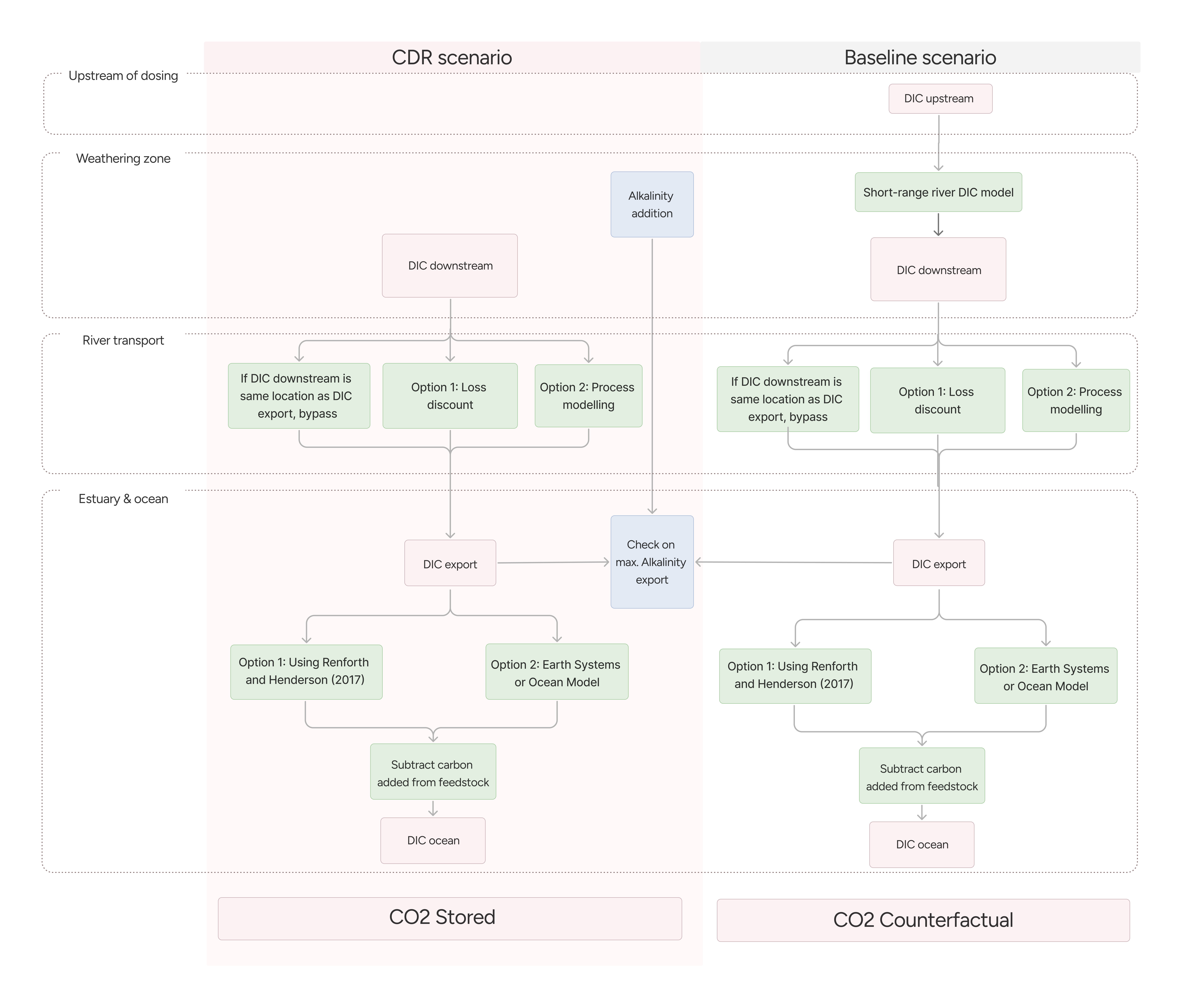
Figure 3. Quantification overview for CO2eStored and CO2eCounterfactual.
Quantification of uncertainty is required for each term in Equation 2 in line with Section 2.5.7 of the Isometric Standard. See Section 5.5.1 for more details.
The quantification framework outlined in the following sections describes a single dosing point for simplicity. However, the framework is also applicable to projects with multiple dosing points along a river. Furthermore, projects that include dosing in different rivers within the same watershed (i.e. all drain to the same river mouth) can be grouped together for verification as a single project with multiple upstream dosing locations. The quantification approach and location(s) of dosing points must be clearly described in the PDD. Any modifications to the quantification approach for multiple dosing locations must be agreed upon in consultation with Isometric
8.2
Calculation of CO₂eStored, RP
The removal of CO2 via RAE occurs at a range of spatial and temporal domains along the river (Figure 4). The initial mixing length is the distance downstream of dosing that it takes for particulate and solute concentrations to disperse into a statistically stable cross-sectional profile. CDR will primarily occur within the weathering zone, the region of the river where feedstock dissolves following the weathering reaction. After the weathering zone, as water travels towards the river mouth, there are processes which may result in additional ingassing or outgassing of CO2. Upon discharge to the ocean, re-speciation of DIC may shift the carbonate equilibrium, altering the final efficiency of the alkalinity increase in the river.

Figure 4: Depiction of spatial domains and quantification steps for River Alkalinity Enhancement. Spatial domains include upstream of dosing, weathering zone, river transport zone, and estuary and ocean. These terms are used throughout to indicate where measurements are required or recommended for quantifying CDR.
The total CO₂ removed from the atmosphere and permanently stored is determined by the cumulative increase in DIC storage in the ocean as a result of RAE. The increase in DIC storage in oceans can be determined by estimating the export of DIC from the river and correcting for ocean re-equilibration losses and carbon added in carbonate feedstocks.
Equation 3
Where
- is the increase in DIC storage in oceans due to river discharge with RAE over the reporting period, in tonnes C.
- is the total export of DIC to the ocean from the river mouth over the reporting period, in tonnes C.
- is the total amount of carbon added as alkaline feedstock over the reporting period, in tonnes C (see Rock and Mineral Feedstock Characterization Module v1.0).
- is the conversion factor between tonnes of carbon to tonnes CO2.
- is a dimensionless term accounting for losses of CO2 due to re-equilibration of DIC upon discharge to the ocean (See Section 8.2.2).
8.2.1
Quantification of DIC Export
The total export of DIC to the ocean from the river mouth, can be calculated as
Equation 4
Where
- is the molar mass of carbon in tonnes/mol;
- is the average DIC concentration at the river mouth over time interval, i, in mol/kg;
- is the average density of water at the river mouth over time interval, i, in kg/m3;
- is the average discharge at the river mouth over time interval, i, in m3/day;
- is the duration of time period, , over which measurements are averaged, in days;
- is the total number of time intervals in the reporting period RP to be summed over;
There may be instances in which direct measurement at the river mouth is not feasible, or does not resolve a sufficient signal, so measurements are taken instead at a location that is downstream of the dosing point. In this case, any additional losses during river transport between the downstream measurement location and the river mouth must be accounted for, and the total DIC export to the ocean can be quantified as
Equation 5
Where
- is the molar mass of carbon in tonnes/mol;
- is the average DIC concentration at the downstream measurement location, over time interval, i, in mol/kg;
- is the average density at the downstream measurement location, over time interval, i, in kg/m3;
- is the average flow rate at the downstream measurement location, over time interval, i, in m3/day;
- is the duration of time period, i, over which measurements are averaged, in days;
- is the total number of time intervals in the reporting period RP to be summed over;
- are losses of CO2 during river transit from the downstream measurement point to the river mouth (see Section 8.2.1.2), dimensionless.
8.2.1.1
Step 1: Quantification of Downstream DIC Fluxes
The downstream measurement point must be beyond the initial mixing length and can be as far downstream as the river mouth. There are tradeoffs depending on where the measurement location is taken:
- Measurements taken within the weathering zone may not capture the full dissolution or equilibration of the alkalinity addition which may result in a lower estimate for CO2e stored or require forward modeling to estimate the dissolution of feedstock.
- Measurements taken immediately following the weathering zone will have the largest signal, but will require modeling a longer reach of the river between the measurement point and the river mouth.
- Measurements taken close to the river mouth may have a smaller signal due to dilution, and require modeling a shorter distance to the river mouth since the measurement captures a larger proportion of the transformations during river transit.
- Measurements taken directly at the river mouth do not require quantification of downstream transformations as they will already be integrated into the measurement, in which case Step 2 can be skipped.
The choice of measurement locations will depend on the length of the river reach, as well as the availability of suitable measurement locations. Multiple measurement locations may be needed for long river reaches to appropriately represent spatial variability along the river.
The measurement signal must be statistically significant and above the estimated downstream [DIC] from the baseline model (see Section 8.3). The Project Proponent must justify the statistical test used, and the significance level must be 0.05 with the null hypothesis being there is no change in between the CDR and baseline scenarios.
See Section 11 for more details on measurement locations and required parameters.
8.2.1.2
Step 2: Quantification of Losses and Transformations During River Transport
This step is required unless measurements in Step 1 are taken directly at the river mouth.
As the newly added alkalinity is transported through rivers and eventually, to the oceans, losses may occur that result in either direct loss of alkalinized river water, direct loss of alkalinity from river water or decreased efficiency of that alkalinity to produce carbon dioxide removal in natural waters. As such, losses along river transport to the river mouth and upon entering the ocean must also be considered. Any losses that cannot be justified as negligible must be quantified as a reduction in the gross carbon removal.
River water which does not get discharged to the ocean, such as through water withdrawal, losing rivers, or flow diversions are also considered direct losses of alkalinized river water.
Alkalinity within river water and/or carbon dioxide removal efficiency may be reduced through processes including sorption onto surfaces or particles, biological uptake, or carbonate precipitation. Changes in ambient pH may result in re-equilibration of DIC or calcium carbonate precipitation. These losses may occur heterogeneously through river transport. Risks of losses may be more pronounced at areas with water inputs with different chemical properties, such as groundwater discharge, surface runoff, tributaries or confluences along the river network.
All projects which utilize river transport models must characterize all water additions and withdrawals throughout the river transit between the downstream measurement location in Step 1 and the river mouth.
8.2.1.2.1
Overview of Riverine Biogeochemical Transformations to be Considered
The section that follows includes an overview of riverine transformations and quantification options for each.
Re-equilibration of DIC
Equilibrium speciation of DIC is primarily dependent on pH, and to a lesser extent temperature, salinity and pressure:
Equation 6
The release of CO2 due to re-equilibration of DIC may occur due to mixing of fluids with different pH. This may occur upon initial dosing of alkalinity, at river confluences and when rivers discharge to the ocean.The recommended quantification approaches for estimating outgassing downstream is through a model that explicitly calculates the change in relevant geochemical properties throughout the river network and is informed by carbonate system measurements collected near the river mouth.
Carbonate precipitation
Secondary precipitation of calcium carbonate could cause CO₂ outgassing by the following reaction:
Equation 7
Calcium carbonate precipitation may result in a reduction in carbon stored by 50% for non-carbonate feedstocks or 100% for carbonate feedstocks. In rivers, higher suspended particulates may increase mineral nucleation. Some research suggests there is a relationship between increased alkalinity loss with higher TSS14. Thus, the risk of secondary precipitation is most pronounced in the vicinity of alkalinity dosing, where the carbonate chemistry and TSS perturbation are largest.
Limiting pH and the saturation state has been shown to be effective at avoiding this result, and laboratory research to characterize the critical thresholds that trigger precipitation under close-to-natural conditions are ongoing 15, 16, 17, 18, 19. Furthermore, precipitation dynamics occur on a timescale between minutes to hours15, 17, which suggests that dilution could be an effective risk mitigation strategy.20
Natural alkalinity flux reduction
Increased alkalinity in rivers can potentially reduce the natural alkalinity flux from river or marine sediments 21. This risk may be exacerbated by projects with settling particles that result in local alkalinity enrichment in marine or river sediments, and the potential impacts on the net removal calculation is uncertain at this time. More research in this area is needed and the Protocol will be updated with future advancements.
Additional (bio)geochemical sinks of alkalinity
Additional (bio)geochemical sinks of alkalinity may be operative in river systems. This may include pH-mediated precipitation of soluble metals, sorption of cations to surfaces or suspended solids or the biological uptake of cations. Some river systems may also have unique risks that are not otherwise addressed in this Protocol. The Project Proponent is required to identify any additional site-specific sinks of alkalinity and take appropriate action to quantify or mitigate the risk of alkalinity loss due to these site-specific sinks.
It is important to note that some feedstocks may contain acid generating constituents like sulfide minerals, which when weathered can decrease a project’s net carbon removal. Project Proponents must incorporate any sources of acidity in the feedstock into their carbon accounting and loss framework. For fast-dissolving sources of acidity, any losses may already be incorporated into measurements of carbonate system variables. For slow-dissolving sources of acidity, it may be appropriate to discount removals in proportion to future acid generation. The methods used to account for acidity generated from the feedstock must be described in the PDD.
Options for quantifying riverine biogeochemical transformations
There are two options available for quantifying the transformations during river transport.
- Option 1: Loss discount
- Loss discount must at minimum include losses due to re-equilibration of DIC and carbonate precipitation from the downstream measurement location through to the river mouth.
- Option 2: Process modeling
- The Project Proponent may opt to do process modeling to account for additional weathering that has not been observed by the downstream measurement and all applicable loss terms.
8.2.1.2.2
Option 1: Loss Discounting Quantification
To account for potential losses along river transport, Project Proponents must estimate potential losses along the river network through measurement or models.
Processes that can lead to losses include:
- Re-equilibration of the DIC system
- Carbonate precipitation
- Direct losses of alkalinized river water (e.g. water withdrawal, flow diversions)
- Any other site-specific losses
The overall loss discount for a RAE project is the product of the loss factors associated with each loss process:
Equation 8
Where:
- is the overall river loss discount, accounting for processes during the transport from the downstream measurement location to the river mouth. This term is dimensionless and represents the total fraction of CO2 retained upon reaching the river mouth.
- is the fraction of CO2 that is retained after a given loss process,
- is the total number of loss processes, dimensionless.
The recommended approach for determining is to develop a conceptual model of river transport losses. Recent publications have outlined modeling approaches that combine baseline river geochemical data, equilibrium modeling of water chemistry and scenarios of terrestrially exported DIC, which may serve as useful references2223.
Model requirements
The minimum requirements for river transport loss models are:
- Domain:
- River network through which alkalinity ions will be transported
- Input River characteristics:
- Calcite saturation index (SIc)
- pH
- pCO₂
- Alkalinity
- Any reductions of river water, e.g. due to water withdrawal, losing rivers, or flow diversions
- Outputs:
- SIc along river*
- pH along river
- for re-equilibration of DIC during river transport
- for carbonate precipitation during river transport
- for direct losses of alkalinized water, if applicable to project, during river transport
Project Proponents are required to submit a detailed description of their modeling approach, including the model used, the river/watershed data used in model construction and the source of that data. Alternate approaches may be considered on a case by case basis.
*Note on calcite saturation index in rivers
Calcite saturation index (SIc) is a useful parameter to determine the likelihood of carbonate precipitation. Calcite saturation index (SIC) is calculated as:
Equation 9
With
Equation 10
Where:
- is the measured solution activities of those ions
- is the ion activities at saturation
A SIc > 0 is considered supersaturated, however, the kinetics of carbonate precipitation are exceeding slow and not typically observed below SIc = 1 23.
8.2.1.2.3
Option 2: Process Modeling
The second option for quantifying riverine transformations is to use a process model that includes all the sources and sinks of alkalinity between the measurement point and the river mouth. This approach may be more desirable if the downstream measurement point is taken within the weathering zone, and the Project Proponent wishes to quantify further weathering and atmospheric re-equilibration during transport to the ocean using a model. Examples of commonly used catchment models that include explicit representation of inorganic carbon are Integrated Catchment Model (INCA)24 and Hydrologic Simulation Program - Fortran (HSPF)25, which could be applied to RAE projects.
Model Requirements
The minimum requirements for the process model are:
- Domain:
- The model must span the region from the downstream measurement point in Step 1, through the river mouth.
- DIC budget:
- The model must include representation of the following sources and sinks of DIC: atmospheric exchange, biological uptake & respiration, interaction with sediments, carbonate precipitation, weathering, additional inputs into the river (e.g. at confluences), and direct losses of river water during transport
- Inputs:
- Downstream measurements from Step 1 should set the initial DIC conditions of the model
- Realistic atmospheric conditions (e.g. air temperature and precipitation) representative of the project region and season should be used as inputs
- Outputs:
- Daily averaged DIC at the river mouth
- Uncertainty
- A list of the major sources of uncertainty must be reported, with the largest source of uncertainty quantified with an ensemble simulation, e.g. varying the inputs across their range to obtain a distribution of output values
- A conservative output value of 1 standard deviation below the mean should be used in the net CDR calculation
Model validation
The process model must meet the following model validation requirements:
- Model results of DIC must be compared against observations of concentrations and carbon fluxes at similar locations along the river (e.g. at the river mouth, or another measurement point downstream the measurement point taken in Step 1). The validation should occur for different seasons, and must include the seasons in which dosing occurs.
- Model validation must be performed for the baseline case, using river measurements collected either pre-deployment or during a period where no dosing occurs.
- It is recommended to also validate the model during the RAE project scenario with some downstream measurements, if there is a detectable signal.
- The model must be re-validated at minimum once every 3 years.
Project Proponents are required to submit a detailed description of their modeling approach, including the model used, the river/watershed data used in model construction and the source of that data. Alternate approaches may be considered on a case by case basis.
8.2.2
Step 3: Quantification of Ocean Losses
Discussion
As alkalinity is transported through the estuary to the ocean, changes in pH, temperature and/or salinity can shift the carbonate system and result in a re-equilibration of DIC. Estimates from peer-reviewed studies suggest that marine losses of terrestrially exported DIC could amount to 10-30% loss of exported carbon, depending on the temperature and pH change between the river and ocean, salinity, pCO₂, and ocean circulation 2,26,27,28,29. Typically, the ocean has a higher pH than rivers and the increased presence of CO32- in oceans can reduce the total storage of terrestrially exported DIC. In addition, changes in salinity and saturation state upon reaching the ocean can lead to calcium carbonate precipitation 30.
Quantification
Outgassing upon entering the ocean must be quantified using regional data specific to the area where the river reaches the ocean. This loss can be estimated with one of the following approaches:
- Using the Renforth and Henderson (2017) uptake efficiency equation
- Using a 3D Earth Systems Model or ocean physical-biogeochemical model to explicitly simulate ocean circulation and air-sea CO2 fluxes in the impacted region (Kanzaki et al., 2023)
Alternative approaches may be considered by the Isometric science team on a case by case basis, provided the approach is sufficiently described and justified in the PDD.
Option 1 assumes thermodynamic equilibrium with the atmosphere and provides an upper limit on the expected ocean losses. Option 2 considers the 3D ocean circulation and does not assume equilibrium with the atmosphere, which may lead to fewer losses in certain regions if the exported DIC is subducted out of atmospheric contact for long periods of time before it has a chance to outgas.
It is a known limitation that both Option 1 and 2 presented do not adequately represent the physical and biogeochemical interactions that occur through transit in the estuarine zone. As such, Option 1 and 2 are specifically catered to systems where mixing will lead to outgassing of CO2 as a result of re-equilibration of DIC at circumneutral pH to the ocean’s slightly basic pH (e.g. pH ~ 8,1).
It is possible that some scenarios may lead to additional CO2 uptake instead of outgassing where the river and ocean mix (e.g., a river with exceptionally high pH). This additional DIC uptake in the ocean is not eligible for crediting under this Protocol. Therefore, , the unitless efficiency term describing the fracton of exported DIC that is retained in the ocean, cannot exceed 1.
An Estuarine CO2 Uptake Module is under development and quantification of the air-water CO2 uptake under the distinct physical and biogeochemical processes occuring within estuaries and will be presented as a third Option in the future.
8.2.2.1
Option 1: Using Renforth and Henderson (2017)
The Renforth and Henderson (2017) uptake efficiency equation for a local water body is:
Equation 11
Where
- is the change in the local ocean total DIC as a result of RAE, in mol/kg
- is the change in the local ocean Total Alkalinity as a result of RAE, in eq/kg
- is the local ocean partial pressure of CO2 at the discharge site, in μatm
- is the local ocean surface temperature, in °C
- is the local ocean salinity, in %
A dimensionless uptake efficiency term, can then be calculated as follows:
Equation 12
Where
- is defined in Equation 11
- is the total export of Alkalinity to the ocean from the river mouth over the reporting period (calculated from Step 2)
- is the total export of DIC to the ocean from the river mouth over the reporting period (calculated from Step 2)
Project Proponents should use the oceanographic conditions from publicly available locationally-specific time-series data, such as the NOAA climate indices list, OceanSODA-ETHZ, or equivalent, to the uptake efficiency (Equation 11). The efficiency can be used in Equation 12 to determine the magnitude of the loss term. Equilibrium conditions can be assumed.
8.2.2.2
Option 2: Earth Systems or Ocean Model
Another approach to quantifying ocean losses is to use a 3D Earth Systems Model or ocean physical-biogeochemical model to explicitly simulate ocean transport and air-sea CO₂ fluxes. For example, Kanzaki et al., (2023) used an Earth system model to estimate the ocean outgassing of CO₂ from terrestrial enhanced weathering projects29. Similar model-based approaches may be used, however the calculation of ocean losses must be regionally specific to the project-site. A globally averaged loss factor may not be used at this time since it may not be conservative, given the large variability that exists in different regions of the ocean.
Projects Proponents must submit a detailed description of their modeling approach in the PDD, including the following:
- the model used and domain
- inputs and forcing data, including atmospheric forcing and initial conditions
- carbonate system representation and parameterization of air-sea CO₂ fluxes
- representation of RAE project, e.g. as represented through an additional flux of DIC and alkalinity into the ocean at a particular river mouth
- baseline simulations
Furthermore, the model must be well-validated and skillful for its intended purpose. Proof of model validation can be achieved through either:
- A track record of use in science, industry, or government applications, which is demonstrated through multiple peer-reviewed papers, or proof of usage in a number of previous applications.
- Newly developed models without a track record of usage must be validated against reputable data sources, which include quality-controlled in situ measurements and public datasets adhering to FAIR (Findable, Accessible, Interoperable and Reusable) principles 31. Sufficient model validation data must be provided with the PDD.
8.3
Calculation of CO₂eCounterfactual, RP
Type: Counterfactual
8.3.1
Counterfactual DIC export to ocean
The naturally occurring export of DIC from the river to the ocean is calculated as:
Equation 13
Where
- is the increase in DIC storage in oceans due to river discharge, in tonnes C.
- is the total export of DIC to the ocean from the river mouth, in tonnes C.
- 44/12 is the conversion factor between tonnes of carbon to tonnes CO2.
- are losses of CO2 due to re-equilibration of DIC upon discharge to the ocean.
The quantification of must use the same approach as the CDR intervention scenario (Equation 3, Section 8.2).
A primary difference is that direct measurements downstream of the dosing location of the counterfactual scenario are not possible. Therefore, quantification of parameters at the downstream measurement location (ie. ) requires measurements upstream of the dosing location paired with a short-range river DIC model developed for the specific river reach.
8.3.1.1
Short-range River DIC Model
The short-range river DIC model can be a statistical model that predicts from other measurable parameters such as river measurements upstream of dosing and/or catchment properties. Inputs to the model must be real-time data of river carbonate chemistry parameters upstream of dosing location. For example, multiple linear regression models have been used to predict carbonate system parameters in rivers from catchment properties 32. More complex deep learning models such as long short-term memory neural networks have also been successfully applied to predicting water quality variables in inland waters 33. It is recommended to use the simplest possible statistical model that yields high-performance.
Model requirements
The short-range river model used to estimate baseline downstream parameters (ie. ) must:
- Be based on peer-reviewed methodologies
- Be trained on high quality data:
- Carbonate chemistry variables must be collected directly from the project area or a close paired-catchment.
- Catchment characterization and hydrologic variables can be from reputable sources (e.g., hydrochemical data from national datasets such as US Geological Survey, Environment Canada; catchment properties from HydroSHEDS).
- Inputs to the model must include real-time carbonate chemistry parameters upstream of the dosing location and span a range of hydrograph, temperature and pH conditions to explore the extremes and event-based nature feedstock weathering and DIC export
- Have a detailed workflow that justifies:
- Model selection and architecture
- Dataset collation and preprocessing
- Model skill assessment based on a test dataset not used for training, including reporting r2, RMSE, bias, and a 1:1 plot of model performance. The model skill assessment must be used to inform a conservative uncertainty discount.
Requirements for model architecture and minimum thresholds for model skill will be updated as the state of science evolves.
Model Validation
The short range river DIC model must be re-validated at minimum every 3 years. It is recommended that the model is routinely revalidated by turning off dosing periodically to collect additional data of downstream baseline conditions and compare against baseline model predictions. Episodic re-validation is recommended after extreme events.
Appropriate Model Use
There must be a check in each verification that the distribution of training data encompasses the range of conditions observed during the Reporting Period (e.g. similar seasons, temperature, upstream pH, etc.). If project conditions are outside the training distribution (e.g. there was a record rainfall month with precipitation values beyond the training data), the model is ineligible for use, unless additional model validation can be demonstrated. The model may need to be retrained or fine-tuned periodically with updated baseline measurements.
The output of the short-range river DIC model is , which can then be used to calculate following the same approaches outlined in Section 8.2.
8.3.2
Counterfactual feedstock weathering
In addition to the counterfactual DIC export from the river to ocean, in some instances it may be appropriate to consider weathering of feedstock that would have occurred without project intervention. For example, if the feedstock used constitutes a waste product that was not mined or quarried specifically for project activities and was stored in open-air conditions, some degree of surficial weathering could be expected over timescales relevant to a project lifetime. Project Proponents using these feedstocks must account for counterfactual weathering if the feedstock does not undergo additional processing prior to deployment. This Protocol defines the durability of a RAE Credit as 1,000+ years; thus, this is the default assumption for the calculation timescale of counterfactual weathering if no additional information regarding the storage conditions and duration of the feedstock at the mine/quarry site can be provided. If additional information on the conditions and duration of feedstock storage at the feedstock supplier are available, Project Proponents may justify calculating the counterfactual across a time period relevant to the specific mine or quarry from which the feedstock is sourced in the PDD. For example, projects operating in conjunction with active mines may find it appropriate to use the time of mine closure and provide details of the closure plan in the PDD. Alternatively, if sufficient documentation exists suggesting that piles of waste materials generated by the feedstock will not be exposed to ambient environmental conditions for a period exceeding a set number of years, the counterfactual may be considered across that time span. It is important to note that studies have shown that the vast majority of weathering in tailings piles occurs in the surface layer that is exposed to the atmosphere, provided that there is no mechanical overturn. For this reason, counterfactual weathering needs to be accounted for in the top meter of the tailings pile.
Where relevant, counterfactual weathering must be calculated by a combination of direct measurements and modeling of the expected weathering rate of feedstock under storage conditions relevant to the source site for either 1,000 years or a time period justified in the PDD as described above. Models must be justified by empirical data from subsamples of the feedstock; guidelines for sampling procedures that adequately capture feedstock heterogeneity are described in the Rock and Mineral Feedstock Characterization Module v1.0. Models must take into account:
- Feedstock mineralogy (required; direct measurement)
- Feedstock surface area (required; direct measurement)
- Baseline carbonation of the tailings pile (required; direct measurement)
- CDR potential of the feedstock (required; calculated from direct measurements of the feedstock batch)
- Environmental conditions of the source site (required; direct measurement or publicly available data), including:
- Temperature
- Average yearly precipitation
- Rainwater pH
- Groundwater pH
- Carbonate saturation
- Permeability (required; direct measurement or calculated from direct measurement)
- Water saturation (required; direct measurement or calculated from direct measurement)
- Microbial activity (recommended; direct measurement)
The measurements and model used to calculate counterfactual feedstock weathering must be provided to Isometric and the VVB. Where counterfactual weathering is considered, is calculated as the sum of counterfactual DIC export to the ocean (Equation 13) and counterfactual weathering of feedstock.
8.4
Validation and Reconciliation Calculations
Project Proponents must conduct the following validation checks each Reporting Period.
Maximum Removal Potential from Alkalinity Flux Assuming full dissolution of the feedstock and no downstream losses, the increased alkalinity export from the river mouth will be the amount of alkalinity added to the river. As a theoretical maximum, the following condition must be true:
Equation 14
If this condition is not met, an audit must be conducted in coordination with Isometric to determine the likely source of the discrepancy.
See the Rock and Mineral Feedstock Characterization Module v1.0 for details on the determination of feedstock alkalinity.
8.5
Calculation of CO₂eGHG Emissions, RP
Type: Emissions
is the total GHG emissions associated with a Reporting Period, . This can be calculated as:
Equation 15
Where
- represents the total GHG emissions for a Reporting Period, in tonnes of CO₂e.
- represents the GHG emissions associated with project establishment, represented for the Reporting Period, in tonnes of CO₂e, see Section 8.5.1.
- represents the total GHG emissions associated with operational processes for a Reporting Period, in tonnes of CO₂e, see Section 8.5.2.
- represents GHG emissions that occur after the Reporting Period and are allocated to a Reporting Period, in tonnes of CO₂e, see Section 8.5.3.
- represents GHG emissions associated with the project’s impact on activities that fall outside of the system boundary of a project, over a given Reporting Period, in tonnes of CO₂e, see Section 8.5.4.
The following sections set out specific quantification requirements for each variable.
8.5.1
Calculation of CO₂eEstablishment, RP
GHG emissions associated with project establishment should include all historic emissions incurred as a result of project establishment, including but not limited to the SSRs set out in Table 1.
Project establishment emissions occur from the point of project inception up until the first Reporting Period. Establishment emissions may be accounted for in the following ways, with the allocation method selected and justified by the Project Proponent:
- as a one time deduction from the first removal
- allocated to removals as annual emissions over the anticipated project lifetime
- allocated per output of product (i.e., per ton CO₂ removed) based on estimated total production over project lifetime
The anticipated lifetime of The Project should be based on reasonable justification and should be included in the Project Design Document (PDD) to be assessed as part of project validation.
Allocation of project establishment emissions to removals must be reviewed at each Crediting Period renewal and any adjustments made. If the Project Proponent is not able to comply with the allocation schedule described in the PDD, e.g. due to changes in delivered volume or anticipated project lifetime, the Project Proponent should notify Isometric as early as possible in order to adjust the allocation schedule for future removals. If that is not possible, the Reversal process will be triggered in accordance with the Isometric Standard, to account for any remaining emissions.
Embodied emissions associated with equipment that is built for CDR purposes but used across multiple CDR Projects owned by the Project Proponent may be shared proportionally across Projects. For example this may be based on total equipment capacity and Projected throughput of all combined Projects. Projections and actual equipment use must be reviewed at each Crediting Period for each Project and adjustments must be made where required. In cases where the Project Proponent ceases operations for all Projects with an outstanding emissions debt, the emissions must be taken out of the buffer pools proportionally for all Projects that used the equipment.
8.5.2
Calculation of CO₂eOperation, RP
GHG emissions associated with should include all emissions associated with operational activities, including but not limited to the SSRs set out in Table 1. In particular for RAE projects, the end-of-life for dosing equipment must be described in the PDD. If the doser is disposed of, the CO2 emissions from this disposal must be included in the calculation of .
emissions must be attributed to the Reporting Period in which they occur. Allocation may be permitted in certain instances, on a case by case basis in agreement with Isometric.
8.5.3
Calculation of CO₂eEnd-of-Life, RP
includes all emissions associated with activities that are anticipated to occur after the Reporting Period, but are directly or indirectly related to the Reporting Period. For example, this could include ongoing sampling activities for Monitoring, Reporting, and Verification (MRV) for the specific deployment (directly related), or end-of-life emissions for the project facilities and equipment (indirectly related to all deployments).
GHG emissions associated with may occur from the end of the Reporting Period onwards, and typically through to completion of project site deconstruction and any other end-of-life activities.
GHG emissions associated with activities that are directly related to each deployment must be quantified as part of that Reporting Period. GHG emissions associated with activities that are indirectly related to all deployments may be allocated in the same ways as set out in .
Given the uncertain nature of emissions, assumptions must be revisited at each Crediting Period and any necessary adjustments made. Furthermore, if there are unexpected emissions associated with a Reporting Period, or The Project as a whole, that occur after the project has ended, then the Reversal process will be triggered to compensate for any emissions not accounted for.
8.5.4
Calculation of CO₂eLeakage, RP
includes emissions associated with a project's impact on activities that fall outside of the system boundary of a project. It includes increases in GHG emissions as a result of The Project displacing emissions or causing a knock on effect that increases emissions elsewhere. As an example, creating a market for feedstocks may generate new revenue in the source sector that alters producer behavior in ways that result in additional GHG emissions.
It is the Project Proponent's responsibility to identify potential sources of leakage emissions, however, for a River Alkalinity Enhancement project the following must be considered as a minimum:
- Feedstock replacement
- Consumables replacement
emissions must be attributed to the Reporting Period in which they occur. Allocation may be permitted in certain instances, on a case by case basis in agreement with Isometric.
8.5.5
Energy Use Accounting
This section sets out specific requirements relating to quantification of energy use as part of the GHG assessment. Emissions associated with energy usage result from the consumption of electricity or fuel.
Examples of electricity usage may include, but are not limited to:
- Operation of process equipment (i.e., pumps, mixers, measurement instruments)
Examples of fuel consumption may include, but are not limited to:
- Handling equipment, such as fork trucks or loaders
The Energy Use Accounting Module v1.2 provides requirements on how energy-related emissions must be calculated in a CDR project so that they can be subtracted in the net CO₂e removal calculation. It sets out the calculation approach to be followed for intensive facilities and non-intensive facilities and acceptable emissions factors.
In alignment with the Energy Use Accounting Module v1.2, the consequential impact of electricity usage on the system it is procured from must be included in calculations for intensive projects, as determined in the Energy Use Accounting Module.
Refer to Energy Use Accounting Module for the calculation requirements.
8.5.6
Transportation Emissions Accounting
This section sets out specific requirements relating to quantification of transportation emissions as part of the GHG Statement.
Emissions associated with transportation include transportation of products and equipment as part of a Reporting Period’s activities. Examples may include, but are not limited to:
- transportation of equipment, feedstock and consumables to the dosing location
- transportation of doser to project site
- transportation and shipping related to collection and analysis of samples
The Transportation Emissions Accounting Module v1.1 provides requirements on how transportation-related emissions must be calculated in a CDR project so that they can be subtracted in the net CO₂e removal calculation. It sets out the calculation approach to be followed and acceptable emissions factors.
Refer to Transportation Emissions Accounting Module for the calculation requirements.
8.5.7
Embodied Emissions Accounting
This section sets out specific requirements relating to quantification of embodied emissions as part of the GHG Statement. Embodied emissions are those related to energy use or other emissions during the manufacture of equipment and materials used in a process.
Examples of project-specific materials and equipment that must be considered as part of the embodied emission calculation include but are not limited to:
- feedstock, consumables and associated equipment produced, constructed and utilized explicitly for the CDR project
- process equipment (i.e., pumps, mixers, measurement instruments)
- equipment related to waste handling and disposal
The Embodied Emissions Accounting Module v1.0 sets out the calculation requirements to be followed including allocation of embodied emissions, life cycle stages to be considered, data sources and emission factors.
Refer to Embodied Emissions Accounting Module for the calculation requirements.
9.0
Storage
Ocean DIC Storage Module
9.1
Marine Dissolved Inorganic Carbon (DIC) Storage
The primary storage reservoir of the CO2 removed through River Alkalinity Enhancement is Dissolved Inorganic Carbon (DIC) in the ocean. The durability and reversal risks of this storage reservoir are discussed in the Dissolved Inorganic Carbon Storage in Oceans Module.
Future versions of this Protocol will include expanded storage options, such as storage of DIC in lakes.
9.2
Buffer Pools
As outlined in Section 2.5.9 of the Isometric Standard, the Buffer Pool is a mechanism used to insure against Reversal risks that may be observable and attributable to a particular project through monitoring.
Based on present understanding, reversals in the global ocean Dissolved Inorganic Carbon (DIC) reservoir will not be directly observable with measurements and attributable to a particular project. Reversals of DIC in the ocean is a system-wide storage uncertainty that should be addressed through further scientific research. Projects applicable to this Protocol are categorized as having a Very Low Risk Level of Reversal according to the Isometric Standard Risk Assessment Questionnaire. The Buffer Pool corresponding to this lowest risk score is 2% and is intended as an additional precaution against unknowns.
For more details on Reversals, refer to Sections 2.5.9 and 5.6 of the Isometric Standard.
10.0
Pre-deployment Requirements
All pre-deployment requirements must be described in the PDD. The requirements are as follows:
- Project Proponents must provide a site description including:
- Watershed characterization: discharge, drainage network, watershed boundary, land use, slope, fluvial morphology, precipitation (e.g., rainfal), and discharge regime
- Affected reach of river, including:
- Dosing site: location, site’s distance from the river mouth
- River reaches downstream of dosing site to the river mouth: river transit time, including transit through major hydrologic features (e.g., lakes, control structures, confluences), saturation state, rating curve
- Ecological characterization: species present, sensitive habitats
- Catchments or river reaches in the region which may be suitable controls
- Existing river monitoring data that will be leveraged for The Project
- Project Proponents must characterize the baseline of relevant parameters for quantification and social and ecological safeguarding (see Table 4 for details on locations):
- river discharge,
- carbonate chemistry parameters (e.g. pH, total alkalinity, DIC and pCO2),
- DIC export from the catchment,
- trace metal concentrations of trace metals that will or may be released into natural waterways,
- ecologically relevant parameters (e.g., DO, TSS, turbidity),
- temperature and salinity,
- frequency of environmental conditions and periods when water quality conditions may be more critical (e.g., seasonal variability).
- Project Proponents must develop a conceptual model of dispersion of alkalinity, to estimate the length of the weathering zone. The length of the weathering zone should depend on turbulent mixing, water velocity, feedstock dissolution rate and water quality characteristics, and will inform downstream monitoring efforts. Sensitivity analysis is required to estimate the bounds of the weathering zone and demonstrate adherence to water quality limits under varying environmental conditions.
- Project Proponents must select alkalinity dosing rates that result in alkalinity release that adhere to safety thresholds and minimize water contamination and accumulation in sediments. It is recommended that safe alkalinity dosing rates are determined through modeling and confirmed through measurement immediately downstream of the weathering zone. Safe dosing limits must be determined based on lowest expected discharge or real-time discharge. Alkalinity dosing schedule should gradually ramp up to the intended dosing rate for continuous discharge.
- Project Proponents must have sufficient remediation plans for restoring water quality conditions prior to discharge in the event that negative environmental impacts result from project activities.
- Project Proponents must develop a short-range river DIC model using pre-deployment data collection to predict counterfactual DIC downstream of the weathering zone. The short-range river DIC model must meet the model requirements described in Section 8.3.1.1.
- Rocks and minerals utilized as feedstock must be sufficiently characterized following Isometric’s Rock and Mineral Feedstock Characterization Module v1.0. These include major and trace elemental abundance, mineralogy, particle size distribution, and surface area.
11.0
Monitoring
A monitoring plan must be established prior to project activities and described in the PDD. The aims of the monitoring plan are to:
- directly measure changes in river chemistry to quantify net carbon removal,
- develop, validate and calibrate river models to quantify the counterfactual scenario and downstream river transformations,
- demonstrate permit compliance,
- monitor environmental conditions, and
- establish processes for adaptive management to ensure that projects stop or modify operations if negative impacts are identified.
The monitoring plan must include details about monitoring duration, frequencies, location, SOPs, sample collection methods, analytical methods, thresholds (if applicable), data reporting and quality assurance/quality control. Analysis and reporting of monitoring data and measurement uncertainties should occur for every Reporting Period. Monitoring guidance and requirements will be updated in alignment with advances in sensor technology which enhance the capacity for measurement and monitoring.
11.1
Monitoring Frequency and Duration
Monitoring must span pre-deployment, dosing and post-dosing (if applicable). For pre-deployment environmental monitoring, Project Proponents must provide a baseline characterization of monitored water chemistry and ecological parameters at the site, which should be sufficiently long and well-resolved to characterize background and seasonal variability. The exact duration and frequency of monitoring will depend on the parameters being measured, as well as site and project specific factors. Listed below are considerations for determining and justifying the monitoring frequency and duration.
The duration of pre-deployment monitoring should consider:
- the timescales of the risks identified in the environmental risk assessment
- dosing period
- site-specific river travel time
- timescales of natural variability and availability of historical data
Likewise, post-dosing environmental monitoring should consider:
- the timescales of the risks identified in the projects environmental risk assessment;
- site-specific river travel time;
- dissolution time.
The monitoring frequency should reflect what is necessary to provide sufficient information about the river location. Some factors which may influence the frequency and intensity of the monitoring plan include:
- operational capacity of The Project. The monitoring frequency may need to be increased at times where the discharge is nearing safety thresholds, permitting thresholds or operational capacity.
- location of the dosing site. The monitoring frequency may be more intensive depending on the sensitivity of natural waters.
- dosing schedule. The monitoring frequency should differ depending on batched discharges vs. continuous discharge, and during dosing ramp-up or dosing rate changes vs. steady state operation.
- seasonality. For projects with seasonally varying action thresholds, more frequent monitoring during seasons with greater environmental risks may be required.
- nature of the feedstock. Projects utilizing mineral or rock feedstocks characterized as having a greater risk of heavy metal and/or trace element release may require more frequent monitoring.
11.2
Monitoring Locations
This Protocol requires and recommends monitoring occur at the locations illustrated in Figure 5. Project Proponents are responsible for determining appropriate monitoring locations, which will be site- and project-specific. It is recommended that Project Proponents use models to plan and optimize sampling design 30.

Figure 5 Monitoring locations for River Alkalinity Enhancement projects referred to throughout this protocol. Exact locations of inputs and outflows from the control volume may look different for projects. Note that monitoring locations for ecosystem safety at sensitive zones along the river to the ocean are not labeled as they are determined on a site-specific basis.
11.2.1
Upstream of Dosing, A
Measurements of natural river conditions just upstream of the dosing location are required to identify upstream changes to the river catchment, confirm the lengths of initial mixing and weathering zone, and as inputs for the baseline model (See Section 8.3).
11.2.2
Feedstock Dosing, B
The total quantity of alkalinity determined by dry feedstock weight must be measured prior to dosing. The total time-duration of dosing, time series of mass flow rate and time series of volumetric flow rate must be continuously monitored throughout the Reporting Period. The fraction of solid and dissolved alkalinity discharged from the doser must be measured, or estimated. Whenever possible, Project Proponents should validate their initial particle dissolution kinetics via direct sampling from the doser (e.g., collecting a grab sample from the discharge pipe, followed by immediate filtration and subsequent analysis of the filter and the filtrate for relevant cation content). The uncertainty in the amount of feedstock added over a Reporting Period must be disclosed.
11.2.3
Downstream of Initial Mixing Length, C
At least one monitoring location downstream of the dosing site is required (C, D, or E).
The downstream location must be downstream of the initial mixing length. The mixing length describes the distance over which river properties mix and become homogenized with respect to the newly added alkalinity. The mixing length depends on flow velocity, channel geometry, turbulence and river features such as meanders and pools. Therefore, the mixing length may change dynamically with environmental conditions. It is recommended that the mixing length is estimated for characteristic seasonal flow rates, and monitoring locations are established to ensure measurements capture solute concentrations that have evenly distributed across the river.
The mixing length may also serve a regulatory purpose in determining the spatial limits over which water quality criteria can be exceeded.
11.2.4
Downstream of Weathering Zone, D
The weathering zone is the reach of the river over which feedstock weathering occurs. Its spatial extent depends on the amount and characteristics of the feedstock, river chemistry (pH, saturation state) and physics (flow velocity, temperature, turbulence). Since only dissolved constituents are measured to quantify , it is recommended that the downstream measurement is taken near the end of the weathering zone where the carbonate chemistry signal will be most pronounced.
11.2.5
River Mouth, E
Measurements at the river mouth are required to constrain . Measurements of both and are used to assess the degree of carbonate chemistry equilibration and are used to quantify the loss factor for ocean losses (see Section 8.2.2).
11.2.6
Estuary or Freshwater Plume, F
Measurements of the freshwater plume may be used to determine ocean losses (see Section 8.2.2). Sites that may be at risk of marine carbonate precipitation may require measurement of aragonite saturation state.
11.3
Measurement Parameters for Quantification
Required river parameters for quantification include: river discharge, temperature, salinity, and carbonate system parameters.
Flow rate can be determined using stage-discharge rating curves. Alternate methods such as site-specific rainfall-runoff models, remote sensing, guaging cameras, or statistical methods to relate ungauged and gauged catchments must be validated and described in the PDD.
Temperature and salinity (or conductivitiy) are necessary for determining physical conditions, and should be co-located with other measured quantities. Two carbonate chemistry parameters (pH, TA, DIC, pCO₂) can be used to characterize the carbonate system. It is a known limitation of using pH and pCO₂ measurements to constrain the full carbonate system that uncertainty can be high34. It is therefore recommended that a third carbonate system measurement is collected and measured to constrain the full carbonate system (including the state of carbonate disequilibrium) and recalibrate autonomous sensors.
11.4
Monitoring for Ecosystem Safety
Project Proponents must conduct an environmental impact assessment (EIA) and develop a project and site-specific ecological monitoring and mitigation strategy (see Section 6.3). Monitoring for ecosystem safety should include the weathering zone, estuary and sensitive locations downstream to be identified and determined on a site-by-site basis.
Dissolved oxygen (DO), turbidity, and total suspended solids (TSS) are required in the weathering zone, where the risk of sudden changes are most pronounced. Monitoring Chl-a, dissolved inorganic nutrients, dissolved organic carbon (DOC) and particulate organic carbon (POC) are also recommended to monitor changes in primary production, nutrient availability and the organic carbon cycle.
Project Proponents are recommended to conduct periodic surveys to monitor ecological changes and potential interactions with species of special concern (IUCN listed, commercially exploited or keystone species). Sampling in biota and sediments for accumulation of heavy metals or contaminants is recommended.
Data collection remains imperative for establishing a foundation for future analysis and enabling the assessment of cumulative impacts of River Alkalinity Enhancement, including assessing co-benefits and restoration impacts. Ecological data must be made publicly available, and the location of where data is stored publicly must be included in the PDD.
Thresholds on environmental monitoring parameters are used to determine safe limits for dosing, mitigate environmental risks and identify negative environmental impact.
Two types of thresholds are used:
- Safety thresholds are imposed on the water quality characteristics and controlled prior to release of alkaline feedstock.
- Action thresholds are measured in the river. Parameters measured are indicators of water quality and/or unintended environmental changes. Action thresholds can be absolute or relative, and can be determined by regulatory limits, relative to natural variability based on historical data or relative to a regional control. For example, the action threshold on pH could be 6.5 < pH < 9 or ±0.2 relative to natural variability, whichever is more conservative. Action thresholds may vary seasonally, and should be consistent with monitoring requirements under official permitting.
Effective implementation of these measures must also be accompanied by a robust monitoring plan to detect negative impacts and stop projects when necessary.
11.4.1
Threshold Violations
Violations are determined based on the threshold type, and specificities of the site, permit and intended activities. For example, exceedance of safety thresholds may be determined by daily mean or max values and exceedance of action thresholds in the mixing zone may be determined by weekly and/or monthly mean or max values. All violations need to be reported, and gaps in monitoring data must be justified.
11.4.2
Enforcement Actions
Credits cannot be issued for time periods without sufficient measurements to demonstrate compliance with action and safety thresholds. The handling of data gaps must be reported in the PDD. Removal activity from discharges that occur during time periods of safety threshold violations will not be eligible for crediting. Action threshold violations must trigger adaptive management plans. Failure to adequately address environmental risks or remediate any harm will lead to a project being subject to Credit cessation.
11.5
Missing Data, Outliers etc.
In some cases, circumstances may occur that result in measurements or data that are missing, incomplete or out of line with expectations given the project design or previous measurements. Similarly, disruptions to the project area and ongoing monitoring (e.g., extreme weather events or equipment failure) may result in missing data, outliers or unexplained results. For the purposes of this Protocol, outliers are defined as data that are more than three standard deviations from the mean (or equivalent percentiles for non-normal distributions). In such instances, the Project Proponent may seek clarification on how the data should be handled. When such instances occur, the details must be reported to the VVB and Isometric as quickly as possible after identification. In such situations, and on a case-by-case basis, Isometric will work to remedy the situation in consultation with the Project Proponent and VVB. Examples of possible remedies include omitting outliers that represent a highly improbable result or replacing missing data with a conservative estimator of a group of samples collected from a nearby and likely representative area.
11.6
Summary of Monitored Parameters
Table 4 below summarizes the required and recommended monitoring parameters. Required measurements indicate the minimum common set of measurements needed for all projects under this protocol. Additional required measurements may be necessary based on specifics of The Project, site and environmental risk mitigation plan.
Table 4. Summary of required and recommended measurements for monitoring. Required measurements indicate the minimum common set of measurements needed for all projects under this protocol. The exact monitoring plan must be described in the PDD, including measurements used to develop and validate models.
| Location | Parameter | Requirement Scope | Reason for Measurement | Methods | Frequency |
|---|---|---|---|---|---|
| Upstream of dosing, A | Q, Discharge rate (m3/day) | Required for all projects | Required for determining volume of water flowing through the river, used in total carbon removal calculation | Stage measurement with stage-discharge relationship, or calibrated rainfall runoff model, or calibrated imaging-based methods. | Ongoing before and throughout deployment, with exact frequency justified in the PDD |
| pCO2 | Required for all projects | Required for quantifying amount of carbon removed | pCO2 sensor | ||
| pH | Required for all projects | Required for confirmation of steady state, quantifying amount of carbon removed, and and adhering to permit limits | pH sensor or discrete bottle samples (see Appendix 1 for more guidance) | ||
| DIC | Required for all projects | Required to assess the local state of carbonate disequilibrium and quantifying amount of carbon removed | Discrete bottle samples | ||
| Alk | Required for all projects | Required to assess the local state of carbonate disequilibrium quantifying amount of carbon removed | Discrete bottle samples | ||
| Temperature | Required for all projects | Required for determining physical conditions and making calculations to fully constrain the carbonate system | Sensor | ||
| Salinity | Required for all projects | Required for determining physical conditions and making calculations to fully constrain the carbonate system | Sensor (e.g., conductivity) | ||
| Total Suspended Solids | Recommended for all projects | Recommended for determining total sediment load, confirming feedstock dissolution and monitoring ecosystem health | Discrete bottle samples and filtering directly onto pre-weighed filter and subsequent measurement of mass change through drying (for example, in an oven) | ||
| Bedload | Recommended for all projects | Recommended for determining total sediment load, confirming feedstock dissolution and monitoring benthic ecosystem health | Sediment trap, sediment sampler | ||
| Trace metal concentration | Recommended based on feedstock used, may be required as part of project-specific environmental risk mitigation strategy | Recommended for water and tissue samples in keystone species to track potential trace and heavy metal accumulation | Discrete bottle and tissue sampling | ||
| Feedstock dosing, B | Alkalinity dosing rate for all projects (L/day, kg/day, or other applicable units) | Required for all projects | Required for determining the total alkalinity introduced as a result of the project activity, needed as an input process model | Sensor or calibrated based on dry feed weight of feedstock and flow rate | Ongoing throughout deployment |
| Fraction of dissolved alkalinity | Required for all projects | Required for determining the fraction of solid and dissolved alkalinity to be input into the process model | May be measured or estimated with a model. Recommended to validate particle dissolution kinetics with grab samples and subsequent filtering and analysis. | ||
| Downstream of initial mixing length, C | Q, Discharge rate (m3/day) | At least one downstream measurement location required | Required for quantifying amount of carbon removed | Stage measurement with stage-discharge relationship | At least once per residence time at the onset of project activities until steady state is reached. Ongoing throughout deployment. |
| pCO2 | Required if C used for carbon removal quantification | Required for quantifying amount of carbon removed | pCO2 sensor | ||
| pH | Required if C used for carbon removal quantification | Required for quantifying amount of carbon removed | pH sensor or discrete bottle samples | ||
| DIC | Recommended if C used for carbon removal quantification | Required for quantifying amount of carbon removed | Discrete bottle samples | ||
| Alk | Recommended if C used for carbon removal quantification | Required for quantifying amount of carbon removed | Discrete bottle samples | ||
| Temperature | Required if C used for carbon removal quantification | Required for determining physical conditions and making calculations to fully constrain the seawater carbonate system | Sensor | ||
| Salinity | Required if C used for carbon removal quantification | Required for determining physical conditions and making calculations to fully constrain the seawater carbonate system | Sensor | ||
| Downstream of weathering zone, D | Q, Discharge rate (L/day) | Required if D used for carbon removal quantification | Required for quantifying amount of carbon removed | Stage measurement with stage-discharge relationship | At least once per residence time at the onset of project activities until steady state is reached. Ongoing throughout deployment. |
| pCO2 | Required if D used for carbon removal quantification | Required for quantifying amount of carbon removed | pCO2 sensor | ||
| pH | Required if D used for carbon removal quantification | Required for quantifying amount of carbon removed | pH sensor or discrete bottle samples | ||
| DIC | Recommended if D used for carbon removal quantification | Required for quantifying amount of carbon removed | Discrete bottle samples | ||
| Alk | Recommended if D used for carbon removal quantification | Required for quantifying amount of carbon removed | Discrete bottle samples | ||
| Temperature | Required if D used for carbon removal quantification | Required for determining physical conditions and making calculations to fully constrain the seawater carbonate system | Sensor | ||
| Salinity | Required if D used for carbon removal quantification | Required for determining physical conditions and making calculations to fully constrain the seawater carbonate system | Sensor | ||
| River mouth, E | Q, Discharge rate (m3/day) | Required for all projects | Required for quantifying amount of carbon removed | Stage measurement with stage-discharge relationship | At high frequency when ramp-up is occuring and shortly after any dosing rate changes are made. Frequency may be lowered when the dosing rate is occurring at a steady state. |
| pCO2 | Required for all projects | Required for quantifying amount of carbon removed | pCO2 sensor | ||
| pH | Required for all projects | Required for quantifying amount of carbon removed | pH sensor or discrete bottle samples | ||
| DIC | Required for all projects | Required for quantifying amount of carbon removed | Discrete bottle samples | ||
| Alk | Required for all projects | Required for quantifying amount of carbon removed | Discrete bottle samples | ||
| Temperature | Required for all projects | Required for determining physical conditions and making calculations to fully constrain the seawater carbonate system | Sensor | ||
| Salinity | Required for all projects | Required for determining physical conditions and making calculations to fully constrain the seawater carbonate system | Sensor | ||
| Within sensitive areas along the river to the ocean, to be determined with community engagement | Dissolved Oxygen | Required for all projects, specific location will depend on dosing plan and permit limits | Required as indicator of general ecosystem health | Sensor or discrete bottle samples | Ongoing before and throughout deployment, with exact frequency justified in the PDD. |
| Total Suspended Solids | Required for all projects, specific location will depend on dosing plan and permit limits | Required for monitoring water quality and quantification. | Discrete bottle samples and filtering directly onto pre-weighed filter and subsequent measurement of mass change through drying (for example, in an oven) | ||
| Turbidity | Required for all projects, specific location will depend on dosing plan and permit limits | Required as part of ecosystem monitoring because elevated turbidity can impact photosynthesis and benthic ecosystem health, and be an indicator of secondary precipitation. | Sensor or discrete water sample | ||
| Bedload | Required for all projects | Required for determining total sediment load, confirming feedstock dissolution and monitoring benthic ecosystem health | Sediment trap, sediment sampler | ||
| Chlorophyll-a | Recommended for all projects, may be required as part of project-specific environmental risk mitigation strategy | Recommended as an indicator of general ecosystem health (phytoplankton primary productivity) | Sensor or discrete water sample | ||
| Dissolved inorganic nutrients | Recommended for all projects, may be required as part of project-specific environmental risk mitigation strategy | Recommended as an indicator of general ecosystem health (available nutrients for primary productivity) and nutrient limitation impacts from secondary precipitation. | Discrete water sample | ||
| Dissolved organic carbon | Recommended for all projects, may be required as part of project-specific environmental risk mitigation strategy | Recommended as an indicator of system level perturbations in non-durable carbon reservoirs. | Discrete water sample | ||
| Trace metal concentration | Recommended based on feedstock used, may be required as part of project-specific environmental risk mitigation strategy | Recommended for water and tissue samples in keystone species to track potential trace and heavy metal accumulation | Discrete bottle tissue sampling |
12.0
Acknowledgments
Isometric would like to thank the following reviewers of this Protocol:
- Joshua Dean, PhD. (University of Bristol)
- Shannon Sterling, PhD. (Dalhousie University)
13.0
Definitions and Acronyms
- ActivityAn activity or process or group of activities or processes that alter the condition of a Baseline and leads to Removals or Reductions.
- AdditionalityAn evaluation of the likelihood that an intervention—for example, a CDR Project—causes a climate benefit above and beyond what would have happened in a no-intervention Baseline scenario.
- BaselineA set of data describing pre-intervention or control conditions to be used as a reference scenario for comparison.
- BiodiversityThe diversity of life across taxonomic and spatial scales. Biodiversity can be measured within species (i.e. genetic diversity and variations in allele frequencies across populations), between species (i.e. the total number and abundance of species within and across defined regions), within ecosystems (i.e. the variation in functional diversity, such as guilds, life-history traits, and food-webs), and between ecosystems (variation in the services of abiotic and biotic communities across large, landscape-level scales) that support ecoregions and biomes.
- Buffer PoolA common and recognized insurance mechanism among Registries allowing Credits to be set aside (in this case by Isometric) to compensate for Reversals which may occur in the future.
- BuyerAn entity that purchases Removals or Reductions, often with the purpose of Retiring Credits to make a Removal or Reduction claim.
- Carbon Dioxide Equivalent Emissions (CO₂e)The amount of CO₂ emissions that would cause the same integrated radiative forcing or temperature change, over a given time horizon, as an emitted amount of GHG or a mixture of GHGs. One common metric of CO₂e is the 100-year Global Warming Potential.
- Carbon Dioxide Removal (CDR)Activities that remove carbon dioxide (CO₂) from the atmosphere and store it in products or geological, terrestrial, and oceanic Reservoirs. CDR includes the enhancement of biological or geochemical sinks and direct air capture (DAC) and storage, but excludes natural CO₂ uptake not directly caused by human intervention.
- Carbon FinanceResources provided to projects that are generating, or are expected to generate, greenhouse gas (GHG) Emission Reductions or Removals.
- Carbon FluxThe amount of carbon exchanged between two or more Reservoirs over a period of time.
- ConservativePurposefully erring on the side of caution under conditions of Uncertainty by choosing input parameter values that will result in a lower net CO₂ Removal or GHG Reduction than if using the median input values. This is done to increase the likelihood that a given Removal or Reduction calculation is an underestimation rather than an overestimation.
- CounterfactualAn assessment of what would have happened in the absence of a particular intervention – i.e., assuming the Baseline scenario.
- Cradle-to-GraveConsidering impacts at each stage of a product's life cycle, from the time natural resources are extracted from the ground and processed through each subsequent stage of manufacturing, transportation, product use, and ultimately, disposal.
- CreditA publicly visible uniquely identifiable Credit Certificate Issued by a Registry that gives the owner of the Credit the right to account for one net metric tonne of Verified CO₂e Removal or Reduction. In the case of this Standard, the net tonne of CO₂e Removal or Reduction comes from a Project Validated against a Certified Protocol.
- Crediting PeriodThe period of time over which a Project Design Document is valid, and over which Removals or Reductions may be Verified, resulting in Issued Credits.
- Dissolved Inorganic Carbon (DIC)The concentration of inorganic carbon dissolved in a fluid.
- Dissolved Organic Carbon (DOC)The concentration of organic carbon dissolved in a fluid.
- Double CountingImproperly allocating the same Removal or Reduction from a Project Proponent more than once to multiple Buyers.
- DurabilityThe amount of time carbon removed from the atmosphere by an intervention – for example, a CDR project – is expected to reside in a given Reservoir, taking into account both physical risks and socioeconomic constructs (such as contracts) to protect the Reservoir in question.
- Emission FactorAn estimate of the emissions intensity per unit of an activity.
- Emission ReductionsLowering future GHG releases from a specific entity.
- Environmental Protection Agency (EPA)A United States Government agency that protects human health and the environment.
- EstuaryThe stretch of tidally influenced river where the river and ocean meet. In this protocol, this region is bounded by the head of tide and the seaward limit of estuarine influence in the ocean.
- FeedstockRaw material which is used for CO₂ Removal or GHG Reduction.
- GHG AssessmentThe process by which all emissions associated with a Project's Removal or Reduction process, including leakages, are accounted for.
- GHG StatementA document submitted alongside Claimed Removals and/or Reductions that details the calculations associated with a Removal or Reduction, including the Project's emissions, Removals, Reductions and Leakages, presented together in net metric tonnes of CO₂e per Removal or Reduction.
- Greenhouse Gas (GHG)Those gaseous constituents of the atmosphere, both natural and anthropogenic (human-caused), that absorb and emit radiation at specific wavelengths within the spectrum of terrestrial radiation emitted by the Earth’s surface, by the atmosphere itself, and by clouds. This property causes the greenhouse effect, whereby heat is trapped in Earth’s atmosphere (CDR Primer, 2022).
- GtCGigatonnes of carbon
- LeakageThe increase in GHG emissions outside the geographic or temporal boundary of a project that results from that project's activities.
- Lossesfor open systems, biogeochemical and/or physical interactions which occur during the removal process that decrease the CO₂ removal .
- MaterialityAn acceptable difference between reported Removals/emissions or Reductions/emissions and what an auditor determines is the actual Removal/emissions or Reduction/emissions.
- ModelA calculation, series of calculations or simulations that use input variables in order to generate values for variables of interest that are not directly measured.
- Monitoring, Reporting, and Verification (MRV)The multi-step process to monitor the Removals or Reductions and impacts of a Project, report the findings to an accredited third party, and have this third party Verify the report so that the results can be Certified.
- ProjectAn activity or process or group of activities or processes that alter the condition of a Baseline and leads to Removals or Reductions.
- Project Design Document (PDD)The document that clearly outlines how a Project will generate rigorously quantifiable Additional high-quality Removals or Reductions.
- Project ProponentThe organization that develops and/or has overall legal ownership or control of a Removal or Reduction Project.
- ProtocolA document that describes how to quantitatively assess the net amount of CO₂ removed by a process. To Isometric, a Protocol is specific to a Project Proponent's process and comprised of Modules representing the Carbon Fluxes involved in the CDR process. A Protocol measures the full carbon impact of a process against the Baseline of it not occurring.
- RegistryA database that holds information on Verified Removals and Reductions based on Protocols. Registries Issue Credits, and track their ownership and Retirement.
- Remote SensingThe use of satellite, aircraft and terrestrial deployed sensors to detect and measure characteristics of the Earth's surface, as well as the spectral, spatial and temporal analysis of this data to estimate biomass and biomass change.
- RemovalThe term used to represent the CO₂ taken out of the atmosphere as a result of a CDR process.
- ReversalThe escape of CO₂ to the atmosphere after it has been stored, and after a Credit has been Issued. A Reversal is classified as avoidable if a Project Proponent has influence or control over it and it likely could have been averted through application of reasonable risk mitigation measures. Any other Reversals will be classified as unavoidable.
- River mouthThe location where the river meets the ocean. In this protocol, the river mouth is defined as the head of tide, where tidal effects begin to influence the river’s flow.
- Sensitivity AnalysisAn analysis of how much different components in a Model contribute to the overall Uncertainty.
- SinkAny process, activity, or mechanism that removes a greenhouse gas, a precursor to a greenhouse gas, or an aerosol from the atmosphere.
- SourceAny process or activity that releases a greenhouse gas, an aerosol, or a precursor of a greenhouse gas into the atmosphere.
- StakeholderAny person or entity who can potentially affect or be affected by Isometric or an individual Project activity.
- StorageDescribes the addition of carbon dioxide removed from the atmosphere to a reservoir, which serves as its ultimate destination. This is also referred to as “sequestration”.
- System BoundaryGHG sources, sinks and reservoirs (SSRs) associated with the project boundary and included in the GHG Statement.
- Total AlkalinityDefined as an excess of proton acceptors over proton donors, which functionally describes the ability of a solution to neutralize acids to the CO₂ equivalence point.
- UncertaintyA lack of knowledge of the exact amount of CO₂ removed by a particular process, Uncertainty may be quantified using probability distributions, confidence intervals, or variance estimates.
- ValidationA systematic and independent process for evaluating the reasonableness of the assumptions, limitations and methods that support a Project and assessing whether the Project conforms to the criteria set forth in the Isometric Standard and the Protocol by which the Project is governed. Validation must be completed by an Isometric approved third-party (VVB).
- VerificationA process for evaluating and confirming the net Removals and Reductions for a Project, using data and information collected from the Project and assessing conformity with the criteria set forth in the Isometric Standard and the Protocol by which it is governed. Verification must be completed by an Isometric approved third-party (VVB).
14.0
Appendix 1: Guidance for High Quality Riverine Data Collection
This Appendix is general for CDR approaches which leverage inland waters including River Alkalinity Enhancement, Wastewater Alkalinity Enhancement, and other related pathways.
14.1
Introduction
Field measurements play an important role in:
- ensuring sufficient and up to date baseline river data
- providing data for calibration and validation of river transport models
- monitoring environmental health during and after project activity
Field measurements may include fixed in-situ sensors, ship-based or autonomous transecting and profiling, discrete bottle sampling, field surveys, aerial imaging and remote sensing. There is significant variability in the specific instruments and field methods that may be used to conduct collect data.
Where field measurements are used to establish site characterization or model validation, Project Proponents must provide thorough documentation on planned and completed field campaigns, including details on the campaign design (spatial and temporal coverage, sampling density, data collection techniques, instrument resolution), metadata, data processing, analytical and statistical techniques, instrument calibration and data quality control. In the sections that follow, we highlight some recommended references and best practices to ensure high quality data generation from field measurements.
Collecting discrete bottle samples alongside continuous autonomous sensor measurements is recommended. Both measurement types offer advantages, for example autonomous sensors can offer wider temporal coverage, while bottle samples are crucial for ground truthing absolute values. Additionally, bottle samples can be used to calibrate drift of long term autonomous sensor deployments.
To facilitate accessibility, transparency and interoperability of research relevant data, data collected from field campaigns must adhere to FAIR data principles (Wilkinson et al., 2016)31.
14.2
Specific Guidance for Bottle Samples
For discrete bottle samples, we refer Project Proponents to the Best Practice Data Standards for Discrete Chemical Oceanographic Observations (Jiang et al., 2023-b)35.
Additional considerations for discrete bottle sampling of carbonate chemistry are discussed in Guide to Best Practices in Ocean Alkalinity Research: Chapter 2 (Seawater carbonate chemistry considerations for ocean alkalinity enhancement research: theory, measurements and calculations) 36.
Recommended analytical methods for bottle samples include:
- Methods for DIC sampling in freshwater: Åberg and Wallin (2014); Wallin et al. (2010)
- Methods for Dissolved Organic Carbon (DOC) sampling: Laudon et al. (2011)
The following methods are approved by the Clean Water Act, EPA:
14.3
Specific Guidance for Sensors
For sensors, Project Proponents are recommended to follow manufacturer provided user manuals for instrument preparation, maintenance, calibration and quality control. Environmental and deployment factors which may affect the quality and interpretation of data (e.g. instrument orientation, interference, presence of bubbles, sediment, and biology) must be described.
Adoption of innovative sensor technologies is encouraged. For novel sensors, additional information that would typically be available from a manufacturer would also have to be provided. These include detection range, resolution, accuracy, performance under different environmental conditions (ie. temperature ranges) and response time. The expected measurement conditions must be within the sensor’s range.
14.3.1
Pre-deployment
Project Proponents must perform instrument calibration before deployment, and recalibrate instruments at an interval recommended by the manufacturer. Calibration curves or equations for the instrument or sensor must be documented. Post-deployment calibration is recommended to account for instrument drift over the deployment duration.
14.3.2
Maintenance During Deployment
Project Proponents must develop a maintenance plan for moored instruments deployed longer than 30 days. This should include plans to clean or replace sensors that may be impacted by biofoul, such as optical sensors, conductivity cells or flow through sensors.
14.3.3
Data Post-processing
Data processing techniques must be documented, including quality control, filtering, despiking and statistical analysis. The recommended quality control process differs between instruments. It is recommended that data be assessed using Data Quality Assessment and Review practices outlined by the USGS.
The quality control manuals for autonomous instruments prepared by the Integrated Ocean Observing System are a recommended resource.
Quality control checks could include:
- completeness of observations
- ordering of data
- check against physically valid limits
- check data obeys physical laws
- checking statistical tests
- checking regularities of space and time variations
USGS Guidelines and Standard Procedures for Continuous Water-Quality Monitors: Station Operation, Record Computation, QA/QC and Data Reporting (USGS 2006). is a recommended resource.
14.4
Specific Guidance for Discharge Measurements
A variety of tool are commonly used to determine discharge. These include:
- Gauging cameras
- Gauging stations
- River level
- Weirs
These methods can be used individually or concert with one another to reduce uncertainty. We recommend that the Project Proponent consult the variety of resources available through the USGS including Discharge Measurements at Gauging Stations and Satellite-based Remote Sensing of River Discharge.
14.5
Considerations for Data Analysis
Wherever possible, it is recommended that the Project Proponent:
- Conduct monitoring at calm water areas
- Collocate measurements (e.g. stream flow and water quality criteria)
- Incorporate tracers to confirm mixing
- Ensure that measurement is representative of cross-sectional average
- Consider diurnal variations when measuring for pH and pCO2, as they may exhibit a significant diurnal range. See Lynch et al., 2010 and de Montety et al., 2011
- Include dissolved oxygen (DO) to isolate pCO2 signal source and river metabolic state
- Consider gas transfer rates in measurement frequency and project design. See Moog and Jirka (1999) and Melching and Flores (1999).
14.6
River Monitoring Examples
Below are some hypothetical examples that are for illustrative purposes only, to demonstrate some of the site and project considerations when determining the appropriate monitoring duration and frequency for a particular parameter and use case.
Example 1
A RAE project is collecting pre-deployment DIC measurements at the river mouth, which will be used to train a baseline model for the net CDR calculation. The key objective is to ensure sufficient data are collected for developing a robust model, which requires that the baseline data is representative of the range of natural variability that the RAE project might experience during deployment. The RAE project plans on dosing continuously only in the summer months. Based on previous studies of this site, stream discharge is strongly negatively correlated with DIC, and the discharge at the river mouth primarily varies seasonally and with weather events. Monitoring duration: Since the RAE project will only operate in the summer months, it is not necessary to characterize the full seasonal variability and it may be sufficient for the pre-deployment data to be collected in the previous summer, with some additional buffer time, e.g. May-September. Expanding the duration of monitoring is beneficial as it can mitigate potential extreme or abnormal climatic events. Monitoring frequency: To capture DIC measurements under a wide range of river discharge rates, the project makes weekly samples, with additional opportunistic samples depending on meteorological conditions such as right before and after a storm.
Example 2
An environmental risk of a RAE project that the local community is concerned about is increased suspended particles in the water column near the dosing location, which could reduce available light in the water column for photosynthesis and reduce oxygen in the river. To monitor and mitigate against this, the RAE project that is operating continuously for 1 year is monitoring TSS near the dosing location, where the impact is expected to be the largest. The project set a safety threshold that TSS cannot exceed 50 mg/L. Monitoring duration: Since the TSS monitoring is meant for assessing ongoing compliance with a safety threshold, and assessing potential impacts, the monitoring duration must span the full time period of the project activity of 1 year. The project decides to continue collecting data for 2 weeks after the cessation of project dosing to study the return to baseline conditions. Monitoring frequency: The main driver of TSS variability at this site is stream discharge, which varies seasonally and with weather events. The project takes a dynamic sampling approach based on when risk is highest of coming close to the TSS safety threshold. As a default, The Project takes biweekly TSS samples, but increases sampling frequency around storm events as well as during the wet season when there is more precipitation.
15.0
Appendix 2: Guidance for High Quality Marine Data Collection
This Appendix is general for marine CDR approaches: Ocean Alkalinity Enhancement (OAE), Direct Ocean Capture (DOC), Wastewater Alkalinity Enhancement
15.1
Introduction
Field measurements play an important role in:
- ensuring sufficient and up to date baseline marine data
- providing data for calibration and validation of ocean models
- monitoring environmental health during and after project activity
Broadly, field measurements may include moored in-situ sensors, ship-based or autonomous transecting and profiling, discrete bottle sampling, field surveys, aerial imaging and remote sensing. There is significant variability in the specific instruments and field methods that may be used to conduct collect data.
Project Proponents must provide thorough documentation on planned and completed field campaigns, including details on the campaign design (spatial and temporal coverage, sampling density, data collection techniques, instrument resolution), metadata, data processing, analytical and statistical techniques, instrument calibration and data quality control. In the sections that follow, we highlight some recommended references and best practices to ensure high quality data generation from field measurements.
Collecting discrete bottle samples alongside continuous autonomous sensor measurements is recommended. Both measurement types offer advantages, for example autonomous sensors can offer wider temporal coverage, while bottle samples are crucial for ground truthing absolute values. Additionally, bottle samples can be used to calibrate drift of long term autonomous sensor deployments.
To facilitate accessibility, transparency and interoperability of research relevant data, data collected from field campaigns must adhere to FAIR data principles (Wilkinson et al., 2016). Project Proponents should follow the data standards and controlled vocabularies described in Guide to Best Practices in Ocean Alkalinity Research: Chapter 13–Data reporting and sharing for ocean alkalinity enhancement research (Jiang et al., 2023). Metadata should be complete according to the NOAA ocean acidification metadata template.
15.2
Specific Guidance for Bottle Samples
For discrete bottle samples, we refer Project Proponents to the Best Practice Data Standards for Discrete Chemical Oceanographic Observations (Jiang et al., 2023-b). Additional considerations for discrete bottle sampling of carbonate chemistry are discussed in Guide to Best Practices in Ocean Alkalinity Research: Chapter 2 (Seawater carbonate chemistry considerations for ocean alkalinity enhancement research: theory, measurements and calculations) (Schulz et al., 2023).
Recommended analytical methods for bottle samples include:
| Parameter | Recommended Method |
|---|---|
| Carbonate Chemistry parameters (pH, DIC, TA) | Guide to Best Practices for Ocean CO2 Measurements |
| Nutrients | Methods of Seawater Analysis |
| Salinity | TEOS-10 |
| Dissolved Oxygen | Methods of Seawater Analysis |
| Chl-a | Welschmeyer 1994 |
| TSS | Methods of Seawater Analysis |
| Trace metals | GEOTRACES cookbook |
The following methods are approved by the Clean Water Act, EPA:
15.3
Specific Guidance for Autonomous Ocean Instruments
For autonomous instruments, Project Proponents are recommended to follow manufacturer provided user manuals for instrument preparation, maintenance, calibration and quality control. Environmental and deployment factors which may affect the quality and interpretation of data, (e.g. instrument orientation, interference, presence of bubbles, sediment, and biology) must be described.
Adoption of innovative sensor technologies is encouraged. For novel sensors, additional information that would typically be available from a manufacturer would also have to be provided. These include detection range, resolution, accuracy, performance under different environmental conditions (ie. temperature ranges) and response time. The expected measurement conditions must be within the sensor’s range.
15.3.1
Pre-deployment
Project Proponents must perform instrument calibration before deployment, and recalibrate instruments at an interval recommended by the manufacturer. Calibration curves or equations for the instrument or sensor must be documented. Post-deployment calibration is recommended to account for instrument drift over the deployment duration.
15.3.2
Maintenance During Deployment
Project Proponents must develop a maintenance plan for moored instruments deployed longer than 30 days. This should include plans to clean or replace sensors that may be impacted by biofoul, such as optical sensors, conductivity cells or flow through sensors.
15.3.3
Data Post-processing
Data processing techniques must be documented, including quality control, filtering, despiking and statistical analysis. The recommended quality control process differs between instruments. Data should be reported using quality control flags consistent with International Oceanographic Data and Information Exchange (IODE) (Bushnell et al., 2019).
The quality control manuals for autonomous instruments prepared by the Integrated Ocean Observing System are a recommended resource.
Quality control checks could include:
- completeness of observations
- ordering of data
- check against physically valid limits
- check data obeys physical laws
- checking statistical tests
- checking regularities of space and time variations
Data Analysis Methods for Physical Oceanography is a recommended resource for statistical analysis methods (Thomson and Emery, 2014).
15.4
Specific Guidance for Tracer Studies
Tracer studies track effluent using a tracer that is either naturally present or added. They can be useful for mCDR projects to:
- characterize DIC-deficient or alkalinity-enhanced plume transport
- validate physical transport in the ocean model via tracking plume movement
- validate alkalinity uptake via dual tracer regression for OAE projects (Project Proponents are not expected to perform dual tracer regression)
Ideal tracers are not harmful to the environment, have near zero background concentration, are conservative or decay very slowly in relation to the duration of field work, mix freely and can be measured in the field at low concentrations. As such, examples of tracers that may be used in Direct Ocean Capture are fluorescent dyes (i.e. rhodamine dye) and gas tracers (SF6, CH3, SF5, 3He).
Fluorescent dye tracers, such as rhodamine dye, are preferable because they can be detected from aerial imaging or high frequency in situ sensors. Rhodamine dye degrades in days to weeks, and can be helpful for characterizing near-field mixing. Gas tracers have a lifespan on the order of years, and can be useful for large scale experiments, however, they have high global warming potential.
Tracers can be injected into the effluent to increase the trackability of the effluent. Alternatively, the tracer dye can be released directly into the water column as a slug release, to help constrain localized dispersion characteristics for coastal models.
If a tracer study is conducted to characterize pCO2-plume transport, the sampling plan must include vertical profiling along transects. A sufficient number of studies are required to produce a sensitivity analysis. Sampling plan, data analysis and interpretation will be evaluated on a case by case basis.
The US EPA Operating Procedure and USGS Procedure for Dye Tracer Measurements are recommended resources.
The following checklist can be referenced for tracer release studies using rhodamine dye to validate an ocean model or characterize plume transport.
Study planning:
- duration of release should give sufficient time for the field team to complete sampling (this will be site specific)
- required tracer quantity should be based on sensor detection limit, effluent flow rate, duration of test and site specific dilution capacity
Materials preparation:
- prepare dye mixture, ensuring the correct units of dye concentration are used
- dye injection pump should be calibrated in lab to confirm desired volumetric dosage rate
- include release rate at different battery levels and temperature
- prepare instrument and site specific calibration curve between dye concentration and effluent concentration
Release:
- if released with effluent, released at a rate proportional to effluent release rate
- if released with effluent, tracer must be added at an adequate mixing length before final discharge
- if released with effluent, sample from an access valve to measure concentration prior to final discharge
- density and velocity matching for effluent or slug release are considered
- no additions after the injection point
Sampling (ship-based or underway system):
- prior to release, conduct spatial salinity and temperature profiling.
- for ship based sampling, sensor should be placed off the bow, firmly braced and clear of bow waves to minimize disturbance due to wake of the vessel.
- positioning via GPS or triangulation should be +/- 2.5m to ensure sampling station. positions and boat tracks are accurate
- for all measurements, record metadata including sample location, time, depth, sensor probe and other visual observations.
- note areas of high concentrations beyond the mixing zone, as this can signal accumulation or recirculation, which cause the effluent to resurface elsewhere.
Data quality and interpretation:
- consider accuracy of positioning data, variation in discharge flow rate, variability in environmental conditions, calibration curve and measurement method in the interpretation of results.
15.5
Ocean Monitoring Frequency and Duration
Monitoring may span pre-deployment, throughout project operations and post-project operations. For pre-deployment environmental monitoring, Project Proponents must provide a baseline characterization of monitored water chemistry and ecological parameters at the site, which should be sufficiently long and well-resolved to characterize background ocean variability. The exact duration and frequency of monitoring will depend on the parameters being measured, as well as site and project specific factors. Listed below are considerations for determining and justifying the monitoring frequency and duration.
The duration of pre-deployment monitoring should consider:
- the timescales of the risks identified in the environmental risk assessment
- duration of CO₂ capture operations
- site-specific residence time
- timescales of natural variability and availability of historical data
Similarly, post-discharge environmental monitoring should consider:
- the timescales of the risks identified in the environmental risk assessment
- site-specific residence time
- timescales of natural variability and availability of historical data
The monitoring frequency should reflect that which is necessary to provide sufficient information about the impacted waters. Some factors which may influence the frequency and intensity of the monitoring plan include:
- operational capacity of the project. The monitoring frequency may need to be increased at times where the discharge is nearing operational capacity.
- location of the discharge. The monitoring frequency may be more intensive depending on the sensitivity of impacted waters.
- duration and intensity of project operations. The monitoring frequency should differ depending on the duration of project operations and more intense monitoring should occur during ramp-up or operational changes vs. steady state operation. The degree of carbonate chemistry perturbation will also determine the frequency of monitoring required for assessing potential ocean losses.
- seasonality. Seasonal variability of the project site. may require more frequent monitoring, particularly during seasons with greater environmental risks.
15.6
Ocean Monitoring Examples
Below are some hypothetical examples that are for illustrative purposes only, to demonstrate some of the site and project considerations when determining the appropriate monitoring duration and frequency for a particular parameter and use case.
Example 1
An OAE project is monitoring for changes in ocean pH near the discharge site to make sure the change in pH does not exceed a threshold of +/-0.2 of the natural variability of pH. The dosing period is 1 week, and the residence time of the region where pH sensors are deployed is 1 day. At this site, it is known from previous studies and published literature that the dominant temporal modes of variability for pH are diurnal and seasonal, due to biological activity. Monitoring duration: Because the activity and dosing period are much shorter than the seasonal variability in this case, it is not necessary for the baseline characterization to span a full year to resolve the seasonal cycle. Instead, the baseline monitoring for a few days before deployment is sufficient. There is ongoing monitoring during the 7 day dosing period, and the post-dosing monitoring for pH should additionally span at least the residence time. To be conservative and to collect additional safety data though, The Project decides to extend post-dosing monitoring for 1 week. Monitoring frequency: To resolve the diurnal cycle variability, sampling should be conducted at a higher frequency than daily, e.g. sampling at minimum every 6 hours would result in at least 4 measurements per day and would be sufficient here. Luckily, The Project uses continuous pH sensors, which allows them to sample much more frequently to fully resolve the diurnal cycle.
Example 2
An environmental risk of a mineral OAE project that the local community is concerned about is bioaccumulation of metals in a nearby oyster farm. To address this, The Project is monitoring the concentration of trace metals in oyster tissues before and after The Project activity. The Project is dosing feedstock particles into the ocean for 1 week, but some of the feedstock will accumulate on the seafloor and it can take up to 3 months for the particles to fully dissolve. The farm grows oysters in the ocean for 1 year before harvesting. Monitoring frequency: The accumulation of any metals in oysters will take some time, especially because it will take a few months after project dosing completes for the feedstock particles to dissolve. Thus it was decided to sample the oysters once a month for the first 3 months following the project activites since that is the period during which particle dissolution is expected to occur, and then once a season after that. Monitoring duration: In this case, the community would like to know the impacts on the oysters that are being harvested for food. So the post-deployment monitoring lasts for 1 year post-dosing (taking seasonal samples) to span the oysters growth cycle and to ensure that metal concentrations do not exceed the local food safety regulatory limits. A control sample was collected from a number of oysters pre-deployment.
16.0
Relevant Works
Footnotes
-
Liu, M., Raymond, P. A., Lauerwald, R., Zhang, Q., Trapp-Müller, G., Davis, K. L., Moosdorf, N., Xiao, C., Middelburg, J. J., Bouwman, A. F., Beusen, A. H. W., Peng, C., Lacroix, F., Tian, H., Wang, J., Li, M., Zhu, Q., Cohen, S., van Hoek, W. J., Li, Y., Li, Y., Yao, Y., and Regnier, P. (2024). Global riverine land-to-ocean carbon export constrained by observations and multi-model assessment. Nature Geoscience, 17, 896–904.https://www.nature.com/articles/s41561-024-01524-z ↩
-
Renforth, P., & Henderson, G. (2017). Assessing ocean alkalinity for carbon sequestration. Reviews of Geophysics, 55(3), 636–674. https://doi.org/10.1002/2016RG000533 ↩ ↩2
-
Huang, W., Cai, W., Wang, Y., Lohrenz, S. E., & Murrell, M. C. (2015). The carbon dioxide system on the Mississippi River‐dominated continental shelf in the northern Gulf of Mexico: 1. Distribution and air‐sea CO2 flux. Journal of Geophysical Research. Oceans, 120(3), 1429–1445. https://doi.org/10.1002/2014JC010498 ↩
-
Li, M., Peng, C., Wang, M., Xue, W., Zhang, K., Wang, K., Shi, G., & Zhu, Q. (2017). The carbon flux of global rivers: A re-evaluation of amount and spatial patterns. Ecological Indicators, 80, 40–51. https://doi.org/10.1016/j.ecolind.2017.04.049 ↩
-
Ludwig, W., Amiotte Suchet, P., & Probst, J.-L. (1996). River discharges of carbon to the world’s oceans: Determining local inputs of alkalinity and of dissolved and particulate organic carbon. Sciences de La Terre et Des Planètes (Comptes Rendus de l’Académie Des Sciences), t. 323, 1007–1014. ↩
-
Mant, R. C., Jones, D. L., Reynolds, B., Ormerod, S. J., & Pullin, A. S. (2013). A systematic review of the effectiveness of liming to mitigate impacts of river acidification on fish and macro-invertebrates. Environmental Pollution, 179, 285–293. https://doi.org/10.1016/j.envpol.2013.04.019 ↩ ↩2
-
Clair, T. A., & Hindar, A. (2005). Liming for the mitigation of acid rain effects in freshwaters: A review of recent results. Environmental Reviews, 13(3), 91–128. https://doi.org/10.1139/a05-009 ↩
-
Bach, L. T., Gill, S. J., Rickaby, R. E. M., Gore, S., & Renforth, P. (2019). CO2 Removal With Enhanced Weathering and Ocean Alkalinity Enhancement: Potential Risks and Co-benefits for Marine Pelagic Ecosystems. Frontiers in Climate, 1, 7. https://doi.org/10.3389/fclim.2019.00007 ↩
-
BS EN 15978:2011 Sustainability of construction works - Assessment of environmental performance of buildings - Calculation method ↩ ↩2 ↩3 ↩4 ↩5
-
Intergovernmental Panel On Climate Change (IPCC) (Ed.). (2023). Climate Change 2022 - Mitigation of Climate Change: Working Group III Contribution to the Sixth Assessment Report of the Intergovernmental Panel on Climate Change (1st ed.). Cambridge University Press. https://doi.org/10.1017/9781009157926 ↩
-
Tian, H., Yao, Y., Li, Y., Shi, H., Pan, S., Najjar, R. G., Pan, N., Bian, Z., Ciais, P., Cai, W.-J., Dai, M., Friedrichs, M. A. M., Li, H.-Y., Lohrenz, S., & Leung, L. R. (2023). Increased Terrestrial Carbon Export and CO2 Evasion From Global Inland Waters Since the Preindustrial Era. Global Biogeochemical Cycles, 37(10), e2023GB007776. https://doi.org/10.1029/2023GB007776 ↩ ↩2
-
Ran, L., Lu, X. X., Yang, H., Li, L., Yu, R., Sun, H., & Han, J. (2015). CO2 outgassing from the Yellow River network and its implications for riverine carbon cycle. Journal of Geophysical Research: Biogeosciences, 120(7), 1334–1347. https://doi.org/10.1002/2015JG002982 ↩
-
Atkins, M. L., Santos, I. R., & Maher, D. T. (2017). Seasonal exports and drivers of dissolved inorganic and organic carbon, carbon dioxide, methane and δ13C signatures in a subtropical river network. Science of The Total Environment, 575, 545–563. https://doi.org/10.1016/j.scitotenv.2016.09.020 ↩
-
Wurgaft, E., Wang, Z. A., Churchill, J. H., Dellapenna, T., Song, S., Du, J., Ringham, M. C., Rivlin, T., & Lazar, B. (2021). Particle Triggered Reactions as an Important Mechanism of Alkalinity and Inorganic Carbon Removal in River Plumes. Geophysical Research Letters, 48(11), e2021GL093178. https://doi.org/10.1029/2021GL093178 ↩
-
Ringham, M., Hirtle, N., Shaw, C., Lu, X., Herndon, J., Carter, B., & Eisaman, M. (2024). A comprehensive assessment of electrochemical ocean alkalinity enhancement in seawater: Kinetics, efficiency, and precipitation thresholds. EGUsphere, 2024, 1–22. https://doi.org/10.5194/egusphere-2024-108 ↩ ↩2
-
Schulz, K. G., Bach, L. T., & Dickson, A. G. (2023). Seawater carbonate chemistry considerations for ocean alkalinity enhancement research: Theory, measurements, and calculations. Guide to Best Practices in Ocean Alkalinity Enhancement Research, 2-oae2023, 2. https://doi.org/10.5194/sp-2-oae2023-2-2023 ↩
-
Moras, C. A., Bach, L. T., Cyronak, T., Joannes-Boyau, R., & Schulz, K. G. (2022). Ocean alkalinity enhancement – avoiding runaway CaCO₃ precipitation during quick and hydrated lime dissolution. Biogeosciences, 19(15), 3537–3557. https://doi.org/10.5194/bg-19-3537-2022 ↩ ↩2
-
Iglesias-Rodríguez, M. D., Rickaby, R. E. M., Singh, A., & Gately, J. A. (2023). Laboratory experiments in ocean alkalinity enhancement research. Guide to Best Practices in Ocean Alkalinity Enhancement Research, 2-oae2023, 5. https://doi.org/10.5194/sp-2-oae2023-5-2023 ↩
-
Suitner, N., Faucher, G., Lim, C., Schneider, J., Moras, C. A., Riebesell, U., & Hartmann, J. (2024). Ocean alkalinity enhancement approaches and the predictability of runaway precipitation processes: Results of an experimental study to determine critical alkalinity ranges for safe and sustainable application scenarios. Biogeosciences, 21(20), 4587–4604. https://doi.org/10.5194/bg-21-4587-2024 ↩
-
He, J., & Tyka, M. D. (2023). Limits and CO 2 equilibration of near-coast alkalinity enhancement. Biogeosciences, 20(1), 27–43. https://doi.org/10.5194/bg-20-27-2023 ↩
-
Bach, L. T. (2024). The additionality problem of ocean alkalinity enhancement. Biogeosciences, 21(1), 261–277. https://doi.org/10.5194/bg-21-261-2024 ↩
-
Zhang, S., Planavsky, N. J., Katchinoff, J., Raymond, P. A., Kanzaki, Y., Reershemius, T., & Reinhard, C. T. (2022). River chemistry constraints on the carbon capture potential of surficial enhanced rock weathering. Limnology and Oceanography, 67(S2), S148–S157. https://doi.org/10.1002/lno.12244 ↩
-
Harrington, K. J., Hilton, R. G., & Henderson, G. M. (2023). Implications of the Riverine Response to Enhanced Weathering for CO2 removal in the UK. Applied Geochemistry, 152, 105643. https://doi.org/10.1016/j.apgeochem.2023.105643 ↩ ↩2
-
Futter, M. N., Butterfield, D., Cosby, B. J., Dillon, P. J., Wade, A. J., & Whitehead, P. G. (2007). Modeling the mechanisms that control in-stream dissolved organic carbon dynamics in upland and forested catchments. Water Resources Research, 43(2). https://doi.org/10.1029/2006WR004960 ↩
-
Bicknell, B. R., Imhoff, J. C., Kittle Jr, J. L., Donigian Jr, A. S., & Johanson, R. C. (1996). Hydrological simulation program—FORTRAN, user’s manual for release 11. US EPA. ↩
-
Fuhr, M., Geilert, S., Schmidt, M., Liebetrau, V., Vogt, C., Ledwig, B., & Wallmann, K. (2022). Kinetics of Olivine Weathering in Seawater: An Experimental Study. Frontiers in Climate, 4. https://www.frontiersin.org/articles/10.3389/fclim.2022.831587 ↩
-
Beerling, D. J., Kantzas, E. P., Lomas, M. R., Wade, P., Eufrasio, R. M., Renforth, P., Sarkar, B., Andrews, M. G., James, R. H., Pearce, C. R., Mercure, J.-F., Pollitt, H., Holden, P. B., Edwards, N. R., Khanna, M., Koh, L., Quegan, S., Pidgeon, N. F., Janssens, I. A., … Banwart, S. A. (2020). Potential for large-scale CO2 removal via enhanced rock weathering with croplands. Nature, 583(7815), 242–248. https://doi.org/10.1038/s41586-020-2448-9 ↩
-
Kantzas, E. P., Val Martin, M., Lomas, M. R., Eufrasio, R. M., Renforth, P., Lewis, A. L., Taylor, L. L., Mecure, J.-F., Pollitt, H., Vercoulen, P. V., Vakilifard, N., Holden, P. B., Edwards, N. R., Koh, L., Pidgeon, N. F., Banwart, S. A., & Beerling, D. J. (2022). Substantial carbon drawdown potential from enhanced rock weathering in the United Kingdom. Nature Geoscience, 15(5), 382–389. https://doi.org/10.1038/s41561-022-00925-2 ↩
-
Kanzaki, Y., Planavsky, N. J., & Reinhard, C. T. (2023). New estimates of the storage permanence and ocean co-benefits of enhanced rock weathering. PNAS Nexus, 2(4), pgad059. https://doi.org/10.1093/pnasnexus/pgad059 ↩ ↩2
-
Mu, L., Palter, J. B., & Wang, H. (2023). Considerations for hypothetical carbon dioxide removal via alkalinity addition in the Amazon River watershed. Biogeosciences, 20(10), 1963–1977. https://doi.org/10.5194/bg-20-1963-2023 ↩ ↩2
-
Wilkinson, M. D., Dumontier, M., Aalbersberg, Ij. J., Appleton, G., Axton, M., Baak, A., Blomberg, N., Boiten, J.-W., da Silva Santos, L. B., Bourne, P. E., Bouwman, J., Brookes, A. J., Clark, T., Crosas, M., Dillo, I., Dumon, O., Edmunds, S., Evelo, C. T., Finkers, R., … Mons, B. (2016). The FAIR Guiding Principles for scientific data management and stewardship. Scientific Data, 3(1), 160018. https://doi.org/10.1038/sdata.2016.18 ↩ ↩2
-
Lauerwald, R., Hartmann, J., Moosdorf, N., Kempe, S., & Raymond, P. A. (2013). What controls the spatial patterns of the riverine carbonate system?—A case study for North America. Chemical Geology, 337, 114-127. ↩
-
Pyo, J., Pachepsky, Y., Kim, S., Abbas, A., Kim, M., Kwon, Y. S., Ligaray, M., & Cho, K. H. (2023). Long short-term memory models of water quality in inland water environments. Water Research X, 21, 100207. https://doi.org/10.1016/j.wroa.2023.100207 ↩
-
Dickson, A.G. Sabine, C.L. and Christian, J.R. (2007) Guide to best practices for ocean CO2 measurement. North Pacific Marine Science Organization, 191pp. (PICES Special Publication 3; IOCCP Report 8). DOI: https://doi.org/10.25607/OBP-1342 ↩
-
Jiang, L., Pierrot, D., Wanninkhof, R. et al. (2023). Best Practice Data Standards for Discrete Chemical Oceanographic Observations. Frontiers in Marine Science. https://www.frontiersin.org/articles/10.3389/fmars.2021.705638/full ↩
-
Schulz, K. G., Bach, L. T., and Dickson, A. G. (2023). Seawater carbonate chemistry considerations for ocean alkalinity enhancement research: theory, measurements, and calculations. State of the Planet, 2-oae2023, 2, https://doi.org/10.5194/sp-2-oae2023-2-2023. ↩
Contributors

Jennifer Yin, Ph.D.

Kevin Sutherland, Ph.D.

Jing He, Ph.D.

Sophie Gill, Ph.D.

Emma Marsland

Isometric
Changelog
River Alkalinity Enhancement © 2025 Isometric HQ Ltd is licensed under CC BY-NC-ND 4.0
Social Safeguards
The Project Proponent must conduct a social impact assessment which adheres to Section 3.7.2 of the Isometric Standard on Social Impacts.
In particular, River Alkalinity Enhancement projects must: