Contents
1.0
Introduction
This Protocol provides the requirements and procedures for the calculation of net carbon dioxide equivalent (CO₂e) removal from the atmosphere via Direct Ocean Capture and Storage (DOCS). DOCS is a marine Carbon Dioxide Removal (CDR) technique that utilizes Direct Ocean Capture technology to capture CO2 in seawater, resulting in a CO2 stream which can be subsequently stored durably (for >1,000 years) in geological reservoirs 1, 2, 3. The CO2-depleted seawater produced during the process is returned to the ocean, which prompts re-equilibration of the atmosphere and surface ocean, resulting in the additional drawdown of atmospheric CO2 and/or a reduction of natural ocean outgassing of CO22, 4.
Direct Ocean Capture is often abbreviated as DOC, however to prevent ambiguity with Dissolved Organic Carbon, this Protocol uses DOCS to describe Direct Ocean Capture and Storage. We also note that this process is sometimes referred to as Direct Ocean Removal (DOR) or Direct Ocean Carbon Capture and Storage (DOCCS).
Direct Ocean Capture uses a pH swing to convert dissolved inorganic carbon (DIC) in seawater into a removable form and then restores the alkalinity of the decarbonated water. In an acid route, temporarily acidified seawater shifts the seawater carbonate equilibrium to higher concentrations of gaseous CO2 which can be captured. Alternatively in a base route, temporarily basified seawater shifts the seawater carbonate equilibrium to higher concentrations of carbonate ions which precipitates it to a solid form as calcium carbonate. Various methods can be used for Direct Ocean Capture, such as, chemical (including electrochemical and photochemical) separation of dissolved inorganic carbon from seawater. Captured CO2 is transported to a durable storage facility for storage on >1000 year timescales. After CO2 capture, the CO2-depleted seawater stream is restored to environmentally safe levels prior to discharge to the ocean. The CO2-depletion in the discharged seawater compared to the natural ocean baseline induces re-equilibration with the atmosphere via air-sea gas exchange which results in a net drawdown of atmospheric CO2 or reduction of natural ocean outgassing.
There are two primary carbon fluxes for DOCS projects: (1) CO2 that is extracted from seawater to storage in a durable reservoir, and (2) CO2 removed from the atmosphere into the surface ocean through air-sea equilibration. Only the storage in reservoir (2) is credited, but storage in reservoir (1) is a prerequisite for the Project to be net-negative and allow for credit issuance. The efficiency of the CO2 removal from the atmosphere through air-sea equilibration must be quantified prior to crediting.
Due to the challenge of using observations at the spatial and temporal scales necessary for quantifying DOCS-induced ocean carbon uptake, the net increase in air-sea CO2 fluxes will be quantified using a validated ocean biogeochemical model, which simulates air-sea equilibration of a DOCS scenario and baseline scenario. More details on model requirements are found in the Air-Sea CO₂ Uptake Module v1.1, and the quantification approach is described in Section 8. Net removal of CO₂e is determined through a GHG Assessment (see Section 7).
Evaluations of the commercial feasibility of DOCS are ongoing and in early stages4, 5. Although abiotic marine CDR methods such as DOCS have promising potential in terms of scalability and efficacy at removing CO₂, scientific understanding around these approaches is currently an active area of research4, 2, 3. As of this writing, there are fewer than 5 DOCS field trials that have occurred or are in the planning stages6, including trials carried out in collaboration between academia and industry. The results of these early stage projects will no doubt shape the future trajectory of DOCS and marine CDR, as well as advance fundamental science in oceanography.
As the first community-level DOCS Protocol for quantifying net CO₂e removal, this Protocol aims to start building consensus around Monitoring, Reporting and Verification (MRV) approaches that are both rigorous and operationally feasible. The guiding principle for this Protocol is to provide a high level of scientific rigor and safety guardrails for early stage DOCS trials and deployments, while also balancing operational feasibility and leaving flexibility for innovation. The aim is achieved here by ensuring the scope of projects that can be credited against this Protocol meet conservative requirements that minimize risks (see Section 4). Furthermore, projects are required to share data relevant for scientific research to facilitate scientific advances in DOCS (see Section 5.5).
Note that throughout this Protocol, use of the word "must" indicates a requirement, whereas "should" indicates a recommendation.
2.0
Sources, Reference Standards and Methodologies
Specific standards and Protocols that are utilized as the foundation of this Protocol, and for which this Protocol is intended to comply with, are the following:
- Isometric Standard 1.0.0
- ISO (International Organization for Standardization) 14064-2: 2019 – Greenhouse Gasses – Part 2: Specification with guidance at the Project level for quantification, monitoring and reporting of greenhouse gas emission reductions or removal enhancements
Additional reference standards that inform the requirements and overall practices incorporated in this Protocol include:
- ISO 14064-3: 2019 - Greenhouse Gases - Part 3: Specification with Guidance for the verification and validation of greenhouse gas statements
- ISO 14040: 2006 - Environmental Management - Lifecycle Assessment - Principles & Framework
- ISO 14044: 2006 - Environmental Management - Lifecycle Assessment - Requirements & Guidelines
Additional standards, methodologies and Protocols that were reviewed, referenced and informed the development of this Protocol include:
- Isometric Direct Air Capture Protocol 1.1.0
- Isometric Ocean Alkalinity Enhancement from Coastal Outfalls 1.0.0
- Criteria for High-Quality Carbon Dioxide Removal, Carbon Direct, Microsoft, 2025
- Guide to Best Practices in Ocean Alkalinity Enhancement Research, Copernicus Publications, State Planet, 2023
- Measurement, Reporting and Verification (MRV) Protocol for OAE Carbon Removal, V3, Planetary Technologies, 2023
- Carbon Dioxide Removal Pathway: Ocean Health and MRV, Captura, 2023
- A Code of Conduct for Marine Carbon Dioxide Removal Research, Aspen Institute, 2021
- BS EN 15978:2011 Sustainability of construction works - Assessment of environmental performance of buildings - Calculation method
- Scientific Background and Fundamentals of MRV: Direct Water Capture, CarbonBlue, 2024
3.0
Future Versions
This Protocol was developed based on the current state of the art, publicly available science regarding DOCS. As DOCS is a novel CDR approach, with limited published literature, the Protocol incorporates requirements that may be highly stringent to minimize risk and for the purposes of environmental and social safeguarding.
This Protocol will be altered in future versions as the science underlying DOCS evolves and the overall body of knowledge and data across all processes is increased, for example regarding feedstock supply, conversion, ecosystem impacts and durable storage.
This Protocol will be reviewed at a minimum every 2 years and/or when there is an update to scientific published literature which would affect net CO₂e removal quantification or the monitoring and modeling guidelines outlined in this Protocol.
4.0
Applicability
As outlined in the Introduction, DOCS projects can be categorized into several different buckets depending on the method of CO2 removal from seawater. This Protocol can be applied to any of the following methods for removing CO2 from seawater:
- Electrochemical separation
- Chemical looping
- Photochemical separation
The aim of this Protocol is to ensure that projects seeking carbon removal Credits for Direct Ocean Capture and Storage are safe and have a demonstrable net-negative climate impact. To be eligible for crediting under this Protocol, projects and associated operations must meet all of the following project conditions.
To ensure safety of human and environmental health, eligible projects must:
- Be officially permitted through relevant regulatory bodies.
- Identify and take action to mitigate environmental and socio-economic risks, as described in Section 3.7 of the Isometric Standard and Section 6 of this Protocol.
To ensure net-negative climate impacts, eligible projects must:
- Be considered additional, in accordance with the requirements of Section 5.4.
- Provide a net-negative CO2e impact (net CO2e removal) as calculated in compliance with Section 8, on a cradle to grave GHG assessment.
- Provide long duration storage (>1,000 yr) of captured CO2 in a durable reservoir and atmospheric CO2 in seawater.
The following applicability requirements are to limit the scope of eligible projects that V1 of this Protocol is developed for. However, these may be expanded in future iterations of the Protocol:
- Projects must be discharging brackish water or seawater depleted in DIC to the surface ocean from a stationary location.
These additional guardrails may be revised in future iterations of the Protocol.
5.0
Relation to Isometric Standard
The following topics are covered briefly in this Protocol due to their inclusion in the Isometric Standard, which governs all Isometric Protocols. See in-text references to the Isometric Standard for further guidance.
5.1
Project Design Document
For each specific project to be evaluated under this Protocol, the Project Proponent must document project characteristics in a Project Design Document (PDD) as outlined in Section 3.2 of the Isometric Standard. The PDD will form the basis for project verification and evaluation in accordance with this Protocol, and must include consideration of processes unique to each DOCS project such as:
- Documentation of official permitting
- Description of pre-deployment activities following Section 10
- Description of the mitigation plan according to the environmental and social risk assessment in adherence with Section 6, including an accompanying robust monitoring plan to ensure efficacy
- Description of the quantification strategy for gross CO2e removal following Section 8
- Description of all measurements and methods used to quantify processes relevant to the calculation of net CO₂e removal, cross-referenced with relevant standards where applicable (see Appendix 2)
- Description of all models used to quantify processes relevant to the calculation of net CO₂e removal that are not directly measurable (see Appendix 3 and Air-Sea CO₂ Uptake Module v1.1)
5.2
Verification and Validation
Projects must be validated and net CO₂e removals verified by an independent third party, consistent with the requirements described in this Protocol as well as in Section 4 of the Isometric Standard.
The Validation and Verification Body (VVB) must adhere to these requisite components:
- verify that the quantification approach adheres to requirements in this Protocol, including demonstration of required records
- verify that the Environmental & Social Safeguards outlined in Section 6 are met
- verify that the Project is compliant with requirements outlined in the Isometric Standard
5.2.1
Verification Materiality
The threshold for Materiality, considering the totality of all omissions, errors and mis-statements, is 5%, in accordance with Section 4.3 of the Isometric Standard.
Verifiers should also verify the documentation of uncertainty of the GHG statement as required by Section 2.5.7 of the Isometric Standard. Qualitative Materiality issues may also be identified and documented, such as (ISO 14064-3: 2019 Section 5.1.7):
- control issues that erode the verifier’s confidence in the reported data
- poorly managed or documented information
- difficulty in locating requested information
- noncompliance with regulations indirectly related to GHG emissions, removals or storage
5.2.2
Site Visits
Project validation and verification must incorporate site visits to project facilities in accordance with the requirements of ISO 14064-3, 6.1.4.2, including, at a minimum, site visits during validation and initial verification. Validators should, whenever possible, observe project operations to ensure full documentation of process inputs and outputs through visual observation (see Section 4 of the Isometric Standard).
A site visit must occur at least once per project validation.
5.2.3
Verifier Qualifications & Requirements
Verifiers and validators must comply with the requirements defined in Section 4 of the Isometric Standard. For this DOCS Protocol, in addition to a primary certified Validation and Verification Body (VVB), independent third party consultants may be required by Isometric for tasks that require subject matter expertise such as the evaluation of suitable ocean models and analysis required in Section 8, Appendix 3, and the Air-Sea CO₂ Uptake Module v1.1. These consultants may be subcontracted out by the VVB or separately contracted by Isometric. Consultants must have relevant experience with the ocean models used in this Protocol, as demonstrated through work experience, post-graduate degrees, research projects, peer-reviewed papers, or equivalent experience.
All VVBs are approved by Isometric independently and impartially based on alignment with Isometric's Conflict of Interest policy, rotation of VVB policy, oversight on quality and the following requirements:
- VVBs must be able to demonstrate accreditation from:
- Alternatively, on a case-by-case basis, if VVBs are able to demonstrate to Isometric that they satisfy all required Verification needs and competencies required for the relevant Protocol and follow the guidelines of ISO 19011 or other relevant standards, they may be approved.
5.3
Ownership
CDR via DOCS can often be a result of a multi-step process, with activities in each step managed and operated by a different operator, company or owner. When there are multiple parties involved in the process, a single Project Proponent must be specified contractually as the sole owner of Credits to avoid double counting of net CO₂e removal. Contracts must comply with all requirements defined in Section 3.1 of the Isometric Standard.
5.4
Additionality
The Project Proponent must be able to demonstrate additionality through compliance with Section 2.5.3 of the Isometric Standard. The baseline scenarios and counterfactuals utilized to assess additionality must be project-specific, and are described in Section 7.2 of this Protocol.
Additionality determinations must be reviewed and completed every 2 years, at a minimum, or whenever project operating conditions change significantly, such as the following:
- regulatory requirements or other legal obligations for project implementation change or new requirements are implemented
- project financials indicate Carbon Finance is no longer required, potentially due to, for example
- increased tipping fees for waste feedstocks
- sale of co-products (such as waste by-product acid) that make the business viable without Carbon Finance
- reduced rates for capital access
Any review and change in the determination of additionality shall not affect the availability of Carbon Finance and Credits for the current or past Crediting Periods, but, if the review indicates the Project has become non-additional, this shall make the Project ineligible for future Credits7.
5.4.1
Uncertainty
The uncertainty in the overall estimate of net CO₂e removal as a result of the Project must be accounted for. The total net CO₂e removal for a specific Reporting Period must be determined with high confidence, and projects must conduct an uncertainty analysis for the net CO₂e removal calculation in compliance with requirements outlined in Section 2.5.7 of the Isometric Standard.
5.4.2
Reporting of Uncertainty
Projects must report a list of all key variables used in the net CO₂e removal calculation and their uncertainties, as well as a description of the uncertainty analysis approach, including:
- required measurements used for net CO₂e removal calculation
- model results from ensemble simulations and/or alternative sensitivity studies
- quantification of model skill through data-model comparisons
- emission factors utilized, as published in public and other databases
- values of measured parameters from process instrumentation, such as truck or pallet weights from weigh scales, electricity usage from utility power meters and other similar equipment
- laboratory analyses
The uncertainty information should at least include the minimum and maximum values of each variable that goes into the net CO₂e removal calculation (see Section 8 for more details). More detailed uncertainty information should be provided if available, as outlined in Section 2.5.7 of the Isometric Standard.
In addition, a sensitivity analysis that demonstrates the impact of each input parameter’s uncertainty on the final net CO₂e removal uncertainty must be provided. Details of the sensitivity analysis method must be provided such that a third party can reproduce the results. Input variables which contribute < 1% change in the net CO₂e removal may be omitted from an uncertainty analysis. For all other parameters, information about uncertainty must be specified.
For more details on model uncertainty, model skill and sensitivity analysis of ocean models, see the Air-Sea CO₂ Uptake Module v1.1 and Appendix 3.
5.5
Data Reporting and Availability
In accordance with the Isometric Standard, all evidence and data related to the underlying quantification of net CO₂e removal and environmental monitoring will be available to the public through Isometric’s Science Platform. That includes:
- Project Design Document (PDD)
- GHG Statement
- measurements taken and supporting documentation, such as calibration certificates
- model specifications and output
- emission factors used
- scientific literature used
The Project Proponent can request certain information to be restricted (only available to authorized Buyers, the Registry and VVB) where it is subject to confidentiality. This includes emissions factors from licensed databases. However, all other numerical data produced or used as part of the quantification of net CO₂e removal will be made available.
In addition, in compliance with the Guide on Data Reporting and Sharing for Ocean Alkalinity Enhancement Research8 and FAIR Principles9, the Project Proponent must publicly disseminate deployment data that is relevant to scientific research (e.g. ocean monitoring measurements, ocean model results), through open access data repositories.
6.1
Overarching Principles
Following the Isometric Standard, Credits issued under this Protocol are contingent on the implementation, transparent reporting and independent verification of comprehensive safeguards. These safeguards encompass a wide range of considerations, including environmental protection, social equity, community engagement and respect for cultural values. The process mandates that safeguard plans be incorporated into all major project phases, with detailed reports made accessible to stakeholders. Adherence to and verification of environmental and socio-economic safeguards is a condition for all Crediting Projects.
For additional guidance and resources on identifying and assessing risk of CDR projects in coastal and marine contexts, we refer Project Proponents to
- Research Strategy for Ocean-based Carbon Dioxide Removal and Sequestration2
- Chapter 2.1 Legal and Regulatory Landscape
- Chapter 2.2 Social Dimensions and Justice Considerations
The following resource on Ocean Alkalinity Enhancement (OAE) may also be relevant for DOCS, although we note that there are differences between the two proceses which may warrant different considerations.
6.2
Governance and Legal Framework
Due to the novelty of marine CDR projects, in many cases, the international, regional and local legal frameworks have yet to catch up with this new industry10, 12, although the EPA has released guidance and frameworks on mCDR permitting structures in the US13. There are also existing regulations on ocean discharges at the international, national, regional and local level that may apply for Direct Ocean Capture and Storage activities. Additionally, specific permits may be required for the installation of an ocean intake, outfall or effluent pipe.
The minimum requirements are:
- Project Proponents must identify jurisdictional authorities, including local rightsholders, of the water body of the Project site and affected areas.
- Project Proponents must receive official permitting for the Project from all relevant authorities of the water body of the Project site and affected areas.
- Project Proponents must observe ratified provisions in international conventions where relevant, and enter into good faith negotiations with Isometric to resolve potential conflicts between applicable regulations and standards. Some examples of potential relevant international conventions are the Convention on the Prevention of Marine Pollution by Dumping of Wastes and Other Matter (“London Convention”) and the Protocol to that Convention (“London Protocol”), the United Nation Convention on the Law of the Sea, the International Convention for the Prevention of Pollution from Ships, the Basel Convention and the European Union Marine Strategy Framework Directive.
6.3
Risk Mitigation Strategies
Environmental and social risk assessment in adherence with Section 3.7 of the Isometric Standard must be completed to identify potential risks, followed by the development of tailored mitigation plans. These plans must encompass specific actions to avoid, minimize or rectify identified impacts. Effective implementation of these measures must also be accompanied by a robust monitoring plan to detect negative impacts and stop projects when necessary (see Section 10).
6.3.1
Environmental Safeguards
The Project Proponent must conduct an environmental risk assessment which adheres to Section 3.7.1 of the Isometric Standard. Specific risks to be considered for DOCS are listed below. The list will be updated in future iterations of the Protocol as new research emerges.
Potential additional environmental risks associated with DOCS are listed below. The severity of these risks vary based on site specificities, and the intensity and duration of marine CDR activities. Environmental and social risk identification, assessment, avoidance, and mitigation planning will be unique to each Project’s technological, environmental, and social contexts. This list is a minimum to which Isometric and the supplier can add risks on a case by case basis, which would be included in the PDD:
Project Proponents must consider the following potential risks associated with mCDR projects as comprehensively as possible, including those in the non-exhaustive list below.
- Generation of co-products and waste must be accompanied by a plan which ensures safe handling, containment and disposal.
- Shock to the ecosystem due to rapid or sudden changes in carbonate system parameters, including termination shock in the case of project cessation.
- Changes in carbonate chemistry, such as pH, could directly help or harm aquatic life depending on the magnitude and direction of the pH shift 14
- Cascading impacts of altered carbonate chemistry, nutrient fields or particle deposition on mineral precipitation, dissolved oxygen, algal blooms, ecosystem community composition and ecosystem functions at and downstream of the receiving water body.
- Disturbances in the riparian and/or coastal zone such as increased erosion from site establishment.
- Impingement, entrainment and entrapment of marine biota from pumping, pre-treatment and the CDR process in projects with seawater intake pipes15, 16.
When assessing marine environmental risks, it is important to holistically consider the context, for instance keeping in mind the Project impacts in relation to the risk of climate change. Projects are not expected to demonstrate zero changes to the ocean ecosystem due to:
- Difficulty in defining the appropriate baseline. The current measured “baseline” in the ocean is rapidly evolving due to climate change. For instance, changes to the ocean state due to climate change increasingly threaten aquatic life through warming temperatures, acidification, increased prevalence of marine disease, mass mortalities and ecological regime shifts.
- Challenges in attributing causation. Observed changes to the marine environment may arise as a result of a CDR project, or from another reason such as a marine heat wave, pollution from a nearby source, etc.
- Risk-benefit analysis of scaling CDR. Scaling CDR technologies, including ocean-based approaches, is critical to meet Paris Agreement targets. Marine CDR technologies are designed to alter the ocean state, so some changes should be expected, particularly at scale.
However, it is important to try to minimize as much as possible any large and/or adverse impacts.
6.3.2
Socio-economic Safeguards
The Project Proponent must conduct a social risk assessment which adheres to Section 3.7.2 of the Isometric Standard on Social Impacts. Marine CDR projects must conduct an environmental justice review, which considers the place-based context of existing coastal infrastructure and marine uses and equitable distribution of coastal amenities and disamenities prior to site selection. Potential disruptions to fisheries, aquaculture, coastal industries, and ocean-based livelihoods must be considered.
6.4
Stakeholder Engagement
Per Section 3.5 of the Isometric Standard, Project Proponents must demonstrate active stakeholder engagement throughout project planning and operation, ensuring that all risk mitigation strategies contribute to sustainable project outcomes. Local stakeholders situated in the vicinity of the Project site may contribute an in-depth understanding of the local system and provide invaluable insights and recommendations on the potential risks, necessary safeguards and specific monitoring needs. Relevant local stakeholders may include local members of academia, Indigenous groups, environmental groups, citizen associations and other users of the marine space, such as commercial and recreational fishermen, shellfish farmers, boaters and recreational users. The Stakeholder Input Process must adhere to requirements outlined in Section 3.5 of the Isometric Standard, and evidence of these meetings must be submitted in the PDD.
6.5
Adaptive Management
Project Proponents must include in the PDD a plan for information sharing, emergency response and conditions for stopping or pausing a deployment. Plans for pausing or stopping a deployment must be in place in instances where:
- instrument malfunctions lead to data-gaps in required monitoring
- effluent exceeds thresholds outlined in the PDD
- regulatory non-compliance, e.g. danger to ecosystem health detected (such as by the local community or government agency)
- compromised health and/or safety of workers and/or local stakeholders
7.0
System Boundary and Project Baseline
7.1
System Boundary & GHG Emissions Scope
The scope of this Protocol includes the GHG sources, sinks, and reservoirs (SSR) associated with a DOCS CDR project.
A cradle-to-grave GHG Statement must be prepared encompassing the GHG emissions relating to the activities outlined within the system boundary.
GHG emissions and removals associated with the Project may be direct emissions from a process or storage system, or indirect emissions from combustion of fuels, electricity generation, or other sources. Emissions must include all GHG SSRs within the system boundary, from the construction or manufacturing of each physical site and associated equipment, closure and disposal of each site and associated equipment, and operation of each process (DOC plant process, CO2 transportation, storage, and monitoring), including embodied emissions of equipment and consumables used in the Project. The Project Proponent is responsible for identifying all sources of emissions directly or indirectly related to project activities.
Any emissions from sub-processes or process changes that would not have taken place without the CDR Project must be fully considered in the system boundary. Any activity that ultimately leads to the issuance of Credits should be included in the system boundary. This allows for accurate consideration of additional, incremental emissions induced by the carbon removal process.
The GHG Statement boundary must include all relevant GHG SSRs controlled, related and affected by the Project, including but not limited to the SSRs set out in Figure 1 and Table 1. If any GHG SSRs within Table 1 are deemed not appropriate to include in the system boundary, they may be excluded provided that robust justification and appropriate evidence is provided in the PDD.
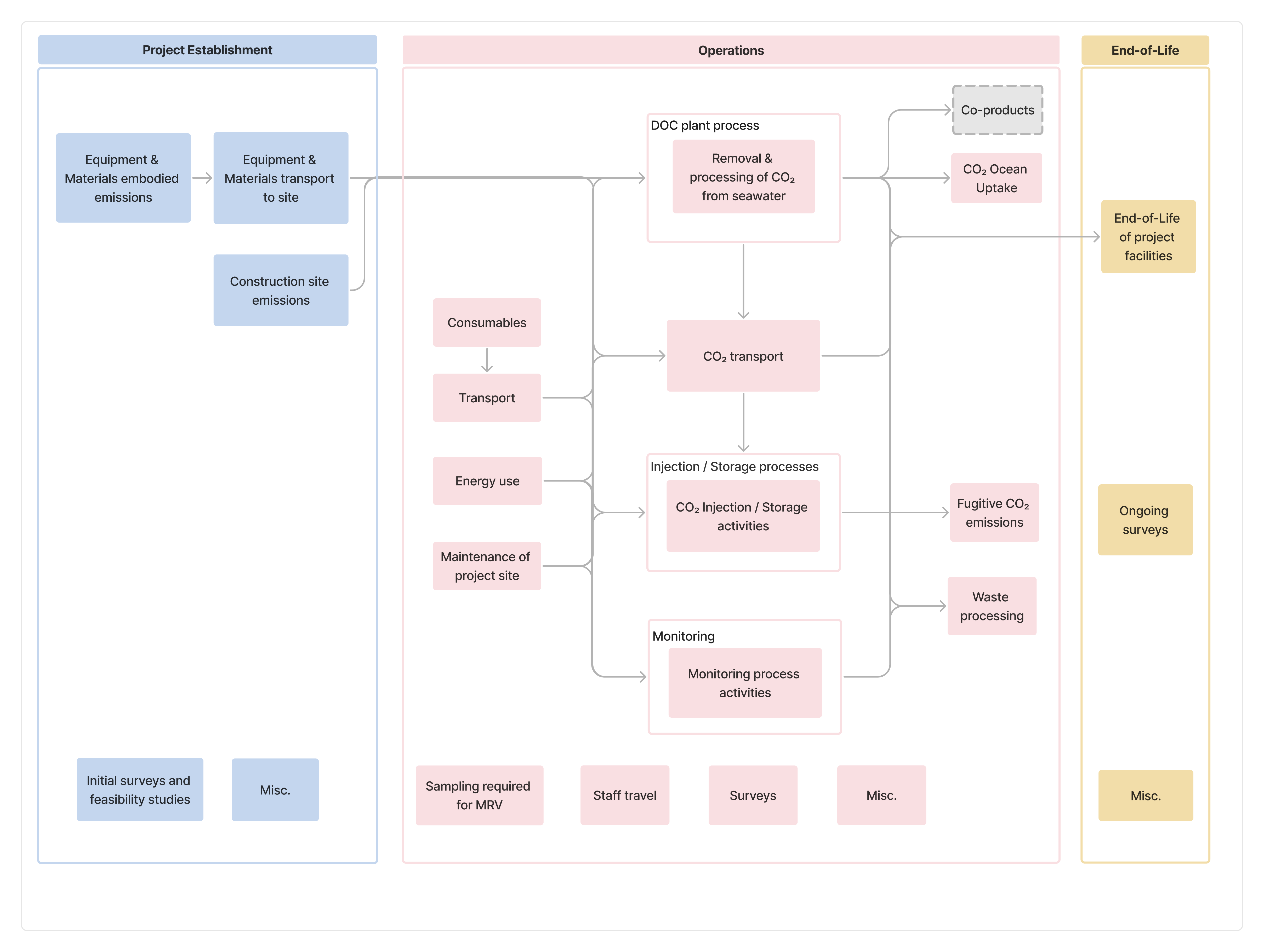
Figure 1. Process flow diagram showing system boundary for DOCS projects.
Table 1. Scope of activities and GHG SSRs to be included by the removal project
| Activity | GHG source, sink or reservoir | GHG | Scope | Timescale |
|---|---|---|---|---|
| Establishment of project | Equipment & Materials embodied emissions | All GHGs | Embodied emissions associated with equipment and materials manufacture for project establishment (lifecycle Modules A1-3). To include product manufacture emissions for equipment, buildings, infrastructure and temporary structures. | Before project operations start - must be accounted for in the first Reporting Period or amortized in line with allocation rules (See Section 8.2.3.1) |
| Equipment and materials transport to site | All GHGs | Transport emissions associated with transporting materials and equipment to the Project site(s) (lifecycle Module A4). | ||
| Construction and installation | All GHGs | Emissions related to construction and installation of the Project site(s) (lifecycle Module A5). To include energy use for construction, installation and groundworks, as well as waste processing activities and emissions associated with land use change. | ||
| Initial surveys and feasibility studies | All GHGs | Any embodied, energy and transport emissions associated with surveys or feasibility studies required for establishment of the Project site. | ||
| Misc. | All GHGs | Any SSRs not captured by categories above. | ||
| Operations | DOC Plant process | All GHGs | Emissions associated with DOC Plant processes including:
| Over each Reporting Period - must be accounted for in the relevant Reporting Period (See Section 8.2.3.2) |
| Transport between DOCS facility and CO2 storage site | All GHGs | Emissions associated with transporting captured CO2 from the DOCS process to a storage facility. | ||
| CO2 Injection / Storage process | All GHGs | Emissions associated with CO₂ injection and storage processes, including:
| ||
| Fugitive CO2 emissions | CO2 | Any captured CO2 that is released back to the atmosphere during or prior to the sequestration process, including as a result of leakage from components, equipment or joints, venting or draining processes, or accidents and equipment failure. | ||
| CO2 Ocean uptake | CO2 | The net amount of CO₂ removed from the atmosphere through air-sea equilibration and durably stored in the ocean as a result of a DOCS project over a Reporting Period. | ||
| Monitoring process | All GHGs | Emissions associated with monitoring, including:
| ||
| Sampling required for MRV | All GHGs | Pre-deployment, deployment and post-deployment monitoring, including transportation to collect samples, shipping of samples for laboratory analysis and sample processing. | ||
| Staff travel | All GHGs | Flight, car, train or other travel required for project operations, including contractors and suppliers required on site. | ||
| Surveys | All GHGs | Embodied, energy and transport emissions associated with undertaking required surveys e.g. ecological surveys. | ||
| Misc. | All GHGs | Any SSRs not captured by categories above. | ||
| End-of-Life | End-of-life emissions | All GHGs | To include anticipated end-of-life emissions (lifecycle Modules C1-4[3]) associated with demolition, deconstruction and waste processing of equipment, buildings or infrastructure. | After Reporting Period - must be accounted for in the first Reporting Period or amortized in line with allocation rules (See Section 8.2.3.3) |
| Ongoing surveys | All GHGs | Embodied, energy and transport emissions associated with undertaking long-term required surveys e.g. ecological surveys. | ||
| Misc. | All GHGs | Any emissions source, sink or reservoir not captured by categories above. |
The Project Proponent must consider all GHGs associated with SSRs, in alignment with the United States Environmental Protection Agency’s definition of GHGs, which includes: carbon dioxide (CO₂), methane (CH4), nitrous oxide (N2O) and fluorinated gasses such as hydrofluorocarbons (HFCs), perfluorocarbons (PFCs), sulfur hexafluoride (SF6) and nitrogen trifluoride (NF3). For CO₂ ocean uptake and fugitive CO₂ emissions, CO2 shall be the only GHG included as part of the quantification. For all other activities, all GHGs must be considered. For example, CO₂, CH4 and N2O are all associated with diesel consumption.
All GHGs must be quantified and converted to CO2e in the GHG Statement using the 100-yr Global Warming Potential(GWP) for the GHG of interest, based on the most recent volume of the IPCC Assessment Report (currently the Sixth Assessment Report)17.
Miscellaneous GHG emissions are those that cannot be categorized by the GHG SSR categories provided in Table 1. The Project Proponent is responsible for identifying all sources of emissions directly or indirectly related to project activities and must report any outside of the SSR categories as miscellaneous emissions.
Emissions associated with a project's impact on activities that fall outside of the system boundary of a project must also be considered. This is covered under Leakage in Section 8.2.3.4.
7.1.1
System Boundary Considerations
7.1.1.1
Ancillary Activities
Ancillary activities are sources of emissions that do not have a direct relationship with the generation of Credits, but are instead required to keep the business operational, or for research and development purposes. The impact of these activities may or may not be significant, depending for example on the life cycle stage of the Project. For rules on Ancillary activities see Section 2.4.2.1 of the GHG Accounting Module v1.0.
See Section 2.4.2.1 of the GHG Accounting Module
7.1.1.2
Facilities with Co-Products
The Project may be reliant on processes occurring separately from the CDR activity, for example, co-locating and making use of desalination plants, cooling water from power plants or other industrial ocean intake pipes or outfalls. DOC processes may also result in the production of co-products.
To allocate project emissions associated with CDR and co-product(s), the Project Proponent may use one or a combination of, where relevant, the co-product allocation procedures. For co-product allocation rules refer to Section 6.1 of the GHG Accounting Module v1.0.
See Section 6.1 of [GHG Accounting Module]
7.1.1.3
Considerations for Waste Inputs
Embodied emissions associated with system inputs considered to be waste products can be excluded from the accounting of the GHG Statement system boundary provided the appropriate eligibility criteria are met.
For waste energy inputs, for example the use of waste heat, refer to the Energy Use Accounting Module v1.2.
Refer to Energy Use Accounting Module for the calculation guidelines.
For all other waste inputs, refer to section 6.3 of the GHG Accounting Module.
See section 6.3 of the GHG Accounting Module.
7.1.1.4
Secondary Impacts on GHG Emissions
DOCS may have additional impacts on GHG emissions beyond the scope of this Protocol. For example there may be potential for a reduction in ocean CO2 uptake as a result of biogeochemical feedbacks in the marine carbon cycle. These potential secondary climate effects are uncertain at this time and are not included in the system boundary.
7.2
Baseline
The baseline scenario for DOCS projects assumes the activities associated with the DOCS project do not take place and any DOCS infrastructure is not built. The counterfactual for DOCS projects considers the CO2 that would have been naturally exchanged with the atmosphere and stored in the ocean in the baseline scenario, over the same spatial and temporal domain as the Project intervention. The counterfactual for DOCS is therefore the background ocean uptake or outgassing of CO₂ over the same spatial and temporal domain as the Project intervention.
8.0
Net CDR Calculation
8.1
Calculation Approach and Reporting Period
The Reporting Period for DOCS represents an interval of time over which removals are calculated and reported for verification. The Reporting Period relates to all activities allocated to an interval of time, including any activities necessary for realizing DIC-removal up until the point of discharge of seawater back into the ocean, as well as activities associated with processing, transport and storage of captured CO2. The total net CO₂e removal is calculated using a combination of measurements and multi-scale modeling for a specified Reporting Period, and is written hereafter as .
8.2
Calculation of CO₂eRemoval
Net CO₂e removal for DOCS for each Reporting Period, RP, must be calculated so as to give high confidence that the estimated net CO₂e was removed.
The net CO₂e removal equation is:
Equation 1
Where
- the total net CO2e removal for Reporting Period RP, in tonnes of CO2e.
- the total CO2 removed from the atmosphere and permanently stored as Dissolved Inorganic Carbon (DIC) in the ocean for a given RP, in tonnes CO2e.
- the total counterfactual CO2 removed from the atmosphere and permanently stored as Dissolved Inorganic Carbon (DIC) in the ocean for a given RP, in tonnes of CO2e.
- the total GHG emissions associated with the Project including leakage, over a given RP, in tonnes of CO₂e.
It should be noted that any potential reversals of CO2 storage in the final storage location occur after Credits have been issued so are not included in this equation. See Section 5.6 of the Isometric Standard for further information. Riak of reversal information is provided in Section 9.
8.2.1
Calculation of CO₂eStored
In a DOCS project, CO2 is removed from the ocean and subsequently durably stored. This results in a decrease in the amount of dissolved inorganic carbon in the ocean, which prompts re-equilibration of the atmospheric and oceanic carbon reservoirs by a net flux of CO2 from the atmosphere to the ocean surface. The gross CO2 removal which is achieved by operation of a DOCS project is determined by the ocean CO2 uptake via air-sea gas exchange minus any fugitive emissions of the captured CO2 from seawater prior to durable storage. The gross CO2 equation is:
Equation 2
Where,
- is the total CO2 absorbed or outgassed from the ocean over the Reporting Period, RP, as a result of the DOCS project, where CO2 that enters the ocean is durably stored as Dissolved Inorganic Carbon (DIC), in tonnes CO2e. This term is positive for CO2 absorbed by the ocean, and negative for outgassing.
- include any captured CO2 from seawater that is released back into the atmosphere prior to sequestration in a durable storage reservoir, over the Reporting Period, RP, in tonnes CO2e.
The counterfactual is given by:
Equation 3
Where
- is the total CO2 absorbed or outgassed from the ocean over the Reporting Period in the counterfactual scenario of no DOCS project, in tonnes CO2e. This term is positive for CO2 absorbed by the ocean, and negative for outgassing.
- include potential miscellaneous emissions in the counterfactual scenario, in tonnes CO2e. This is expected to be zero for qualifying projects in this Protocol.
It is useful to define the following term to represent the net ocean uptake of atmospheric CO2 relative to the counterfactual scenario. Note that throughout this Protocol, will be used to symbolize a difference between the DOCS scenario and counterfactual scenario:
Equation 4
Substituting Equations 2-4 into Equation 1, and assuming , allows Equation 1 to be re-written as
Equation 5
Where
- is defined in Equation 4 and represents the total gross CO2 removal relative to the counterfactual scenario over the Reporting Period, in tonnes CO2e. This term is always positive, representing an increase in CO2 uptake or a decrease in ocean outgassing as a result of the DOCS project.
- include any captured CO2 from seawater that is released back into the atmosphere prior to sequestration in a durable storage reservoir, over the Reporting Period, RP, in tonnes CO2e.
- the total GHG emissions associated with the Project including leakage, over a given RP, in tonnes of CO₂e.
Equation 5 is the primary form of the removal quantification equation that will be used throughout the rest of the Protocol. The following sections provide details on how each of the terms in Equation 5 are calculated.
Quantification of uncertainty is required for each term in Equation 5 in line with Section 2.5.7 of the Isometric Standard. See Section 5.4.1 for more details.
8.2.1.1
Calculation of ΔCO₂eAirSeaFlux
Type: Ocean Storage
Ocean CO2 uptake via DOCS involves processes that span a wide, continuous range of spatial and temporal scales. The quantification framework for the net air-sea CO2 uptake relative to the counterfactual scenario requires explicit characterization of four spatio-temporal regimes depicted in Figure 2. At the smallest scales, the DIC-depleted seawater stream is released into the ocean at the outlet of the DOCS facility, causing a decrease in the seawater pCO2 at this location. Over seconds to hours, in the mixing zone, the plume mixes and moves as its initial momentum is dissipated. Over hours to years, the DIC-depleted water within the surface mixed layer, which may have spread over several hundred kilometers, experiences additional oceanic carbon uptake from the atmosphere or reduction in outgassing via air-sea gas exchange. Air-sea gas exchange may span the near-field (e.g. coastal) and far-field (e.g. open ocean) domains. In the near-field domain, the DIC-depleted water moves and mixes due to nearshore processes such as tides, coastal currents, and waves. Whereas, in the far-field domain, the DIC-depleted water is primarily transported horizontally by regional to basin-scale currents and vertically by upwelling and/or downwelling and turbulent mixing.
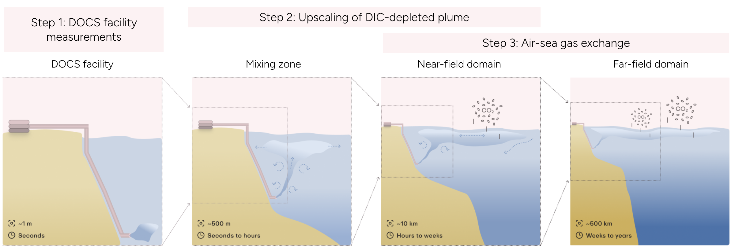
Figure 2 Schematic of the four spatio-temporal regimes (DOCS facility, mixing zone, near-field, far-field) that need to be characterized for the calculation of net air-sea CO2 uptake corresponding with the three quantification steps. Shown here, DIC-depleted seawater discharged at depth generates a buoyant plume which initially rises and mixes in the mixing zone. Air-sea gas equilibration in the coastal and open ocean domains facilitate additional ocean CO₂ uptake or reduces natural ocean outgassing, leading to a net reduction of atmospheric CO2. The spatial scales encompassed by each domain will vary depending on the site and intended activity. Note: a buoyant plume is used for illustrative purposes, other coastal discharge infrastructure, such as surface outfalls, may be used.
This Protocol requires to be determined in three steps, corresponding to the different spatio-temporal regimes above. These steps are summarized below and detailed in the subsequent sections:
- Step 1: Determination of CO2-capture rate is required via direct measurements of the CO2 stream and DIC-depleted seawater.
- Step 2: In the mixing zone and near-field domain, the DIC-depleted seawater is upscaled to a forcing function that can be used in the model used to quantify air-sea CO2 uptake. A number of options are available to complete this upscaling step.
- Step 3: Ocean modeling in the coastal and/or open-ocean domain is used to determine the subsequent air-sea equilibration to quantify .
See Appendix 3: Supplementary Figures for a graphical summary of these steps.
All models used for quantification must be validated in line with Section 2.5.5 of the Isometric Standard. For numerical ocean models used in this Protocol, additional requirements and guidance are provided in Appendix 2 and the Air-Sea CO₂ Uptake Module v1.1.
The quantification framework for is written for projects that reduce pCO2, but do not impact Total Alkalinity (TA). Projects which alter TA of seawater will require some adjustments to the above quantification approach. The same general steps can be followed, but with alterations to account for the TA that is altered. Adjustments to the quantification approach must be agreed upon with Isometric.
8.2.1.1.1
Step 1: Measurements of Seawater Carbon Capture
Relevant Regime: DOCS facility
The initial CDR perturbation induced by a DOCS process is calculated using measurements in the captured CO2 stream, and influent and effluent seawater to determine the cumulative CO2 capture from seawater and the time series of DIC-depleted seawater release.
Measurements must be described in the PDD, and include details about sampling methods, sampling frequency, instrument calibration, data reporting and quality assurance/quality control (see Section 11 for Measurement and Monitoring Requirements). Analysis and reporting of monitoring data and measurement uncertainties should occur for every Reporting Period.
Captured CO2 Stream
CO2 captured from the DOCS process can be calculated with the cumulative mass and average concentration of CO2 captured over time, summed across the whole 𝑅𝑃:
Equation 6
Where:
- is the total amount of CO2 captured from seawater through the DOCS process over the Reporting Period, , in tonnes CO2e
- is the measured concentration of CO2, as weight percent (%wt)
- is the measured mass of CO2 stream, in tonnes
- is the time index, ranging from 1 to 𝑇
- is the number of time units in the Reporting Period, 𝑅𝑃
- is the time interval the average is taken over
For more information on CO2 stream measurement requirements, see Section 11.2. The uncertainty in the amount of CO2 captured over a Reporting Period must be reported.
Influent and Effluent Measurements
Influent measurements are taken prior to any pre-treatment of seawater and CO2 extraction, and effluent measurements taken prior to release to the ocean. Measurements of the influent and effluent are required to obtain a time series of DIC-depleted seawater (e.g. μmol/kg/hour). The total time-duration of discharge and the time series of volumetric flow rate must be continuously measured before being released into the ocean. The uncertainty in the amount of DIC-depletion over a Reporting Period must be reported. See Section 11.3 for more details on measurement requirements.
Step 1 validation Check
The captured CO2 stream measurement must be checked against the DIC-depletion measurements between the influent and effluent. If the captured CO2 stream measurement mean is outside the two standard deviation envelope of the DIC-depletion measurement uncertainty band, an audit must be conducted to determine the most likely source of the discrepancy.
8.2.1.1.2
Step 2: Upscaling of DIC-depleted plume
Relevant Regime: mixing zone and near-field domain
A coastal dynamics study is needed to characterize transport and mixing of the DIC-depleted plume by ambient currents and turbulence. This enables upscaling of the CDR intervention, which may occur over a small region of space, to a time-variable CDR forcing function applied to the ocean model used to quantify air-sea CO₂ uptake.
There are some processes which may occur in the near-field domain that result in losses which must be considered in the determination of the CDR forcing function applied to the ocean model used in Step 3.
In the ocean model, DIC-depletion should be applied as a 3-D interior forcing. Typically, to maximize the atmospheric CO2 drawdown effect, the DIC-depleted plume should be located at or close to the surface ocean, but this may not always be the case. Thus, the vertical distribution of the DIC-depleted waters is important to carefully characterize for the CDR forcing function. Laterally, the shape of the CDR forcing can be represented as a Gaussian or similar parametric form. The results of the coastal dynamics study should be the time-variable 3D CDR forcing function to be applied to the model used for quantifying CO2 uptake, along with its uncertainty.
Ways to determine the time-variable CDR forcing function include:
- Using a validated coastal model to simulate the immediate dispersal of the CDR intervention at the plant location. See Appendix 2 for more details on coastal model requirements.
- Conducting seasonal tracer studies at the deployment site and measuring the depth profile of the tracer in multiple locations in the coastal domain. See Appendix 1 for guidance on tracer studies.
- Demonstrating through a sensitivity study that the ocean model used to quantify air-sea CO₂ uptake is not sensitive to different vertical distributions and temporal variability of the CDR forcing profile, and/or use the input profile that leads to a conservative amount of CO₂ removed. For example, this option would include obtaining a distribution of the net CO2 removal obtained from an ensemble of model simulations where the vertical profile of the CDR forcing is varied.
Hybrid approaches that combine multiple options above, or alternative novel approaches are welcome provided they are well-described and justified, and will be assessed by Isometric on a case-by-case basis. For any of the upscaling approaches used, the uncertainty of the resulting CDR forcing function must be determined. For some projects, a TA forcing function may also need to be obtained using a similar approach.
Project Proponents must consider and disclose the following in the PDD when determining the time-variable CDR forcing function:
- Time series of CO2 capture rate and the total amount of DIC-depletion over the Reporting Period, based on measurements (see Step 1: Effluent measurements above)
- Results of mixing zone model (if using a validated coastal model)
- The density of the effluent relative to the density profile of the receiving waters
- The depth at which the effluent is discharged
- Environmental conditions (e.g. currents, waves, winds)
- Processes that could cause losses
Step 2 validation check
The decrease in DIC represented in the CDR forcing function must be less than or equal to the amount of CO2 captured from seawater, as measured in Section 8.2.1.1.1.
Near-field losses
Upon discharge of DIC-depleted, TA-restored effluent in the ocean, the following processes may occur or change relative to the baseline, which may reduce the efficiency of Direct Ocean Capture:
- CO2 outgassing from secondary precipitation
- CO2 outgassing from biotic calcification
- changes in natural DIC and TA fluxes or buffering of natural TA release from interactions of effluent with sediments
If it cannot be justified that these losses are negligible, it is expected that these losses are quantified and subtracted from the CDR forcing function, since models used to upscale the DIC-depleted plume and to quantify the air-sea CO₂ removal vary in the degree to which they represent the losses, if at all18.
Understanding these and potential other loss terms is an active area of scientific research, and the list of known losses in this Protocol and quantification approach will be updated as research evolves. In the PDD, Project Proponents must describe the risk of these losses, as well as a strategy for quantifying them or a justification of why the losses are negligible. Due to the difficulty and uncertainty in quantifying the impact of these processes at this time, acceptable treatment of loss terms in this Protocol include:
- avoiding the likelihood of these losses by identifying avoidance strategies around conditions which lead to non-negligible loss terms, with corresponding monitoring to demonstrate adherence to those guardrails
- estimating a conservative upper limit of the loss process based on scientific literature, first principles calculations, and/or experimentation
- process-based modeling studies
- direct measurements
- alternative approaches that are sufficiently justified
Data, measurements and evidence used in the quantification of losses must be publicly disclosed. Example recommendations for each loss term are discussed below. Much of the existing research in these loss terms have been motivated by OAE, and may not simulate the carbonate chemistry state of the effluent from eligible DOCS projects. Project Proponents are recommended to conduct research on these loss terms in the relevant carbonate chemistry parameter space for their specific process.
Secondary Precipitation
Secondary precipitation of calcium carbonate in seawater could cause CO₂ outgassing. In the open ocean, abiotic calcium carbonate precipitation is rare because spontaneous nucleation is strongly inhibited in seawater19, 20, 21, and most carbonate production is thought to be biologically mediated22. There are very few areas of the ocean where spontaneous carbonate precipitation is observed (e.g. the Great Bahama Bank and the Persian Gulf22. Such locations typically have exceptionally high saturation states (i.e. ΩCaCO3 > 19)23. In coastal areas, higher suspended particulates may increase nucleation. Early research suggests there is a relationship between increased alkalinity loss due to precipitation andwith higher TSS in the receiving water body24. In the effluent pipe, pipe roughness can also increase potential nucleation sites. Thus, the risk of secondary precipitation is most pronounced in the effluent pipe, mixing zone and coastal domain, where the carbonate chemistry perturbation and potential nucleation sites are largest, and decreases further away from the DOCS discharge location.
Limiting pH and the aragonite saturation state has been shown to be effective at avoiding this result, and laboratory research to characterize the critical thresholds that trigger precipitation under close-to-natural conditions are ongoing25, 26, 27, 28. Furthermore, precipitation dynamics occur on a timescale between minutes to hours (or days) 25, 27, which suggests that dilution could be an effective risk mitigation strategy29 , 30.
An example avoidance strategy is setting a pH threshold, with consideration of TA, TSS and dilution at the site, using a model to guide operations to stay below thresholds (see Pre-deployment) and continuous monitoring of pH, TA, and TSS to ensure that conditions for secondary precipitation are avoided (see Monitoring). Thresholds should be justified by academic literature or laboratory and field analysis of site-relevant characteristics.
In some cases, secondary precipitation can be identified by an observed increase in turbidity. Monitoring of turbidity as an indicator offor secondary precipitation is recommended, however it may be difficult to isolate a signal from secondary precipitation over natural fluctuations. Monitoring for alkalinity for periods of anomalously low alkalinity can also help identify occurrences of secondary precipitation.
Biotic Calcification
Increases in biotic calcification can cause CO₂ outgassing. The carbonate chemistry conditions promoted by Direct Ocean Capture could promote calcification due to the lowered H+/ elevated saturation state31, 32, 33, 34.
Early stage research manipulating Total Alkalinity with the aim of simulating OAE has found no significant increase in biologically produced calcium carbonate at elevated alkalinity in the ocean 35, 36. However, the Black Sea, a naturally elevated alkalinity environment, harbors extensive blooms of the coccolithophores 37, 38, a major group of calcifying plankton. This is thought to be due to the favorable carbonate chemistry promoted by the elevated alkalinity regime34.
This is still an area where more research is needed, particularly through mesocosm and field trials, albeit there is a rich body of literature on lab and mesocosm scale species-specific responses to changing seawater carbonate chemistry (e.g, see Bach et al. (2013) New Phytologist, Bach et al. (2015) Progress in Oceanography, Gafar et al.(2018) Frontiers in Marine Science and others). The risk of alkalinity loss due to biotic calcification may be project and location specific. Recently published meta-analyses synthesizing data from ocean acidification studies for OAE support this claim that species and functional group specificity is likely39. Coastal areas with significant benthic calcification of CaCO3 sediments may be especially susceptible to this feedback.
One potential avoidance strategy is for Project Proponents to set thresholds on pH and TA and monitor for changes in ocean biota. Thresholds should be justified by academic literature or laboratory analysis of site-relevant characteristics. For example, a recent study used lab experiments on representative species of two biogeochemically important phytoplankton functional groups to assess sensitivity to biotic calcification under limestone-inspired OAE conditions35. This study suggests pH < 9 and ΔTA < 1000 μmol/kg as thresholds below which biotic calcification was avoided under the particular conditions studied. Similar studies targeting site relevant water chemistry, the specific CDR perturbation, and calcifying population can be used to determine relevant site and project specific thresholds.
Interactions with Sediments
Early research suggests that altering local carbonate chemistry conditions may reduce natural alkalinity fluxes from sediments40. More research in this area is needed and the Protocol will be updated with future advancements.
A recommended avoidance strategy for DOCS projects is to limit changes in pH and TA near the sea bed through careful design of discharge rates and infrastructure. Thresholds on pH and TA at the sea bed should be justified by academic literature or laboratory analysis of site-relevant characteristics for the specific deployment site. Acceptable evidence for quantification could include measuring benthic alkalinity fluxes and measuring changes in net calcification at the sea bed.
8.2.1.1.3
Step 3: Air-Sea CO₂ Uptake
Relevant Regime: near-field domain and far-field domain
Once the DIC forcing function for the model used to quantify air-sea CO2 uptake is obtained, can be calculated according to the Air-Sea CO₂ Uptake Module v1.1.
Air-Sea CO2 Uptake Module
The air-sea CO2 equilibration must be quantified over the coastal domain, the open-ocean domain, or both. However, it is not required for air-sea gas exchange to be quantified over the initial transport and mixing of the DIC-depleted plume in the coastal domain. This represents a more conservative approach to quantifying CO₂ uptake as the initial air-sea exchange is expected to be large due to the enhanced pCO₂ deficit before full dilution, and there are increased uncertainties regarding air-sea flux parameterizations in coastal areas on short timescales41. If quantification of Removals in the coastal domain is desired, then the coastal domain model must meet the requirements of the Air-Sea CO₂ Uptake Module v1.1. In addition, appropriate care must be taken to ensure connectivity and no double counting of Removals between the coastal and open-ocean domains. This could be accomplished for example with multiscale nested models, or appropriate upscaling of the coastal CO₂ uptake as an additional DIC forcing in the open-ocean model. These approaches must be described in the PDD and will be assessed on a case-by-case basis.
Step 3 Validation check
The total CO₂ removed through air-sea gas exchange must be less than or equal to the amount of CO2 captured from seawater, as measured in Section 8.2.1.1.1.
8.2.1.2
Calculation of CO₂eFugitive Emissions
Release of captured CO2 back into the atmosphere prior to sequestration into a durable storage reservoir is treated as a fugitive emission which must be subtracted from the Removal quantification. These fugitive emissions are calculated as the difference between CO2 captured from the DOCS process and CO2 sequestered in a durable storage well.
Equation 8
Where:
- is the total amount of CO2 captured from seawater through the DOCS process over the Reporting Period, , in tonnes CO2e
- is the total amount of CO2 sequestered in a durable storage reservoir, i, following an applicable storage Module, over the Reporting Period, RP, in tonnes CO2e. This term must be measured following the requirements in the respective storage Module.
- is the total number of durable storage reservoirs used for storage of captured CO2.
The following storage options may be used:
8.2.2
Calculation of CO₂eCounterfactual
Type: Counterfactual
For DOCS, the ocean baseline air-sea CO₂ fluxes are accounted for (see Equations 3–5) and are incorporated in the term in Equation 5. A reminder of the notation used throughout this Protocol is that represents a difference between the DOCS intervention and counterfactual scenarios, with positive values indicating a net increase in marine CO2 storage over the counterfactual scenario.
8.2.3
Calculation of CO₂eEmissions
Type: Emissions
is the total GHG emissions associated with a Reporting Period, RP. This can be calculated as:
Equation 7
Where
- represents the total GHG emissions for a Reporting Period, in tonnes of CO₂e.
- represents the GHG emissions associated with project establishment, represented for the Reporting Period, in tonnes of CO₂e, see Section 8.2.3.1.
- represents the total GHG emissions associated with operational processes for a Reporting Period, in tonnes of CO₂e, see Section 8.2.3.2.
- represents GHG emissions that occur after the Reporting Period and are allocated to a Reporting Period, in tonnes of CO₂e, see Section 8.2.3.3.
- represents GHG emissions associated with the Project’s impact on activities that fall outside of the system boundary of a project, over a given Reporting Period, in tonnes of CO₂e, see Section 8.2.3.4.
The following sections set out specific quantification requirements for each variable in Equation 7.
8.2.3.1
Calculation of CO₂,eEstablishment
GHG emissions associated with should include all historic emissions incurred as a result of project establishment, including but not limited to the SSRs set out in Table 1.
Project establishment emissions occur from the point of project inception through to before the first removal activity takes place. GHG emissions associated with project establishment may be amortized over the anticipated project lifetime, or per output of product. Rules on amortization are outlined in Section 7 of the GHG Accounting Module v1.0 .
See Section 7 of the GHG Accounting Module
8.2.3.2
Calculation of CO₂eOperations
GHG emissions associated with should include all emissions associated with operational activities, including but not limited to the SSRs set out in Table 1.
emissions occur over the Reporting Period for the deployment being credited and are applicable to the current deployment only. emissions must be attributed to the Reporting Period in which they occur.
8.2.3.3
Calculation of CO₂eEnd-of-Life
includes all emissions associated with activities that are anticipated to occur after the Reporting Period, but are directly or indirectly related to the Reporting Period. For example, this could include ongoing sampling activities for MRV for the specific deployment (directly related), or end-of-life emissions for the Project facility (indirectly related to all deployments).
GHG emissions associated with may occur from the end of the Reporting Period onwards, and typically through to completion of project site deconstruction and any other end-of-life activities.
GHG emissions associated with activities that are directly related to each deployment must be quantified as part of that Reporting Period. GHG emissions associated with activities that are indirectly related to all deployments may be allocated in the same ways as set out in .
Given the uncertain nature of emissions, assumptions must be revisited at each Crediting Period and any necessary adjustments made. Furthermore, if there are unexpected emissions associated with a Reporting Period, or the Project as a whole, that occur after the Project has ended, then the Reversal process described in Section 5.6 of the Isometric Standard will be triggered to compensate for any emissions not accounted for.
When the Project Proponent is planning to cease operations within a given storage site, they must project the calculation of monitoring emissions required for post-closure monitoring, and allocate them to the remaining removals taking place at the storage site. If that is not possible, the Project Proponent should allocate those emissions to other projects and/or storage sites they conduct removal operations at, in agreement with Isometric. If for any reason emissions are not appropriately allocated, the Reversal process will be triggered in accordance with Section 5.6 of the Isometric Standard, to account for any remaining monitoring emissions.
In instances where monitoring activities are shared between entities, for example if multiple suppliers use the same storage infrastructure and share monitoring activities, the emissions associated with these activities must be allocated proportionally between the entities in proportion to their contribution towards the overall usage of the storage site by all suppliers.
8.2.3.4
Calculation of CO₂eLeakage
includes emissions associated with a project's impact on activities that fall outside of the system boundary of the Project. It includes increases in GHG emissions as a result of the Project displacing emissions or causing a knock on effect that increases emissions elsewhere. As an example, creating a market for feedstocks may generate new revenue in the source sector that alters producer behavior in ways that result in additional GHG emissions.
It is the Project Proponent's responsibility to identify potential sources of market leakage emissions. For a DOCS project, replacement emissions of consumables used must be considered at minimum. Project Proponents may also consider the impact of project operations on water, land use change and increased strain on existing CO2 transportation and storage infrastructure.
emissions must be attributed to the Reporting Period in which they occur. Allocation may be permitted in certain instances, on a case by case basis in agreement with Isometric.
8.3
Emissions Accounting
8.3.1
General
GHG accounting must be undertaken in alignment with the GHG Accounting Accounting Module v1.0, which ensures a consistently rigorous standard in how GHG emissions are quantified and reported between different CDR Projects and approaches.
Refer to GHG Accounting Module for emissions accounting guidelines.
8.3.2
Energy Use Accounting
This section sets out specific requirements relating to quantification of energy use as part of the GHG Statement. Emissions associated with energy usage result from the consumption of electricity or fuel.
Examples of activities that may require electricity usage may include, but are not limited to:
- operation of process equipment (i.e., pumps, mixers, blowers, flow control, measurement instruments)
- operation of equipment related to intake and pre-treatment of seawater
- electricity for temporary acidification of seawater and CO₂ extraction
- electricity used for the basification/ restoration of water quality pre-discharge and discharge of seawater to the marine environment
- electricity for temporary CO₂ storage
- electricity for CO₂ processing or conversion, such as ex-situ carbonate production and handling
- electricity used for injection operations, including any pumps, compressors (including for compression into supercritical CO₂), or related equipment inside the injection facility gate
- electricity used for non-mobile CO₂ transport
- electricity used for monitoring equipment operation, including analyzers, instrumentation, on-site laboratories specifically for monitoring activities
- electricity used for sampling pumps, sampling systems, or other similar monitoring activities
- electricity used for off site analytical laboratory operation and sample analysis
- electricity for building operation & management for monitoring facility buildings
Examples of activities that may require fuel consumption may include, but are not limited to:
- thermal energy generation (heat/steam)
- cryogenic processes for CO₂ purification or liquefaction
- non-mobile CO₂ transport
- sampling system operation, such as any pumps or heating systems
- handling equipment, such as fork trucks or loaders
- backup generators
- fuel consumption of sampling vessels
The Energy Use Accounting Module v1.2 provides guidance on how energy-related emissions must be calculated in a CDR project so that they can be subtracted in the net CO₂e removal calculation. It sets out the calculation approach to be followed for intensive facilities and non-intensive facilities and acceptable emissions factors.
Refer to Energy Use Accounting Module for the calculation guidelines.
8.3.3
Transportation Emissions Accounting
This section sets out specific requirements relating to quantification of transportation emissions as part of the GHG Statement.
Emissions associated with transportation include transportation of products and equipment as part of a project's activities within a Reporting Period. Examples may include, but are not limited to:
- transportation of consumables to the DOCS location
- transportation and shipping related to collection and analysis of samples for environmental monitoring
- transportation of compressed gaseous or liquid CO₂ or CO₂-containing injectant (such as a carbonate slurry) or carbonated minerals, via freight transportation services, such as rail, truck, or maritime transport
- transportation of samples for lab analysis
The Transportation Emissions Accounting Module v1.1 provides guidance on how transportation-related emissions must be calculated in a CDR project so that they can be subtracted in the net CO₂e removal calculation. It sets out the calculation approach to be followed and acceptable emissions factors.
Refer to Transportation Emissions Accounting Module for the calculation guidelines.
8.3.4
Embodied Emissions Accounting
Embodied GHG emissions associated with the manufacturing, delivery, and installation of all equipment and consumables that lie within the system boundary must be accounted for in each Reporting Period. Embodied emissions are those related to the life cycle impact of equipment and materials used in a process.
Examples of project-specific materials and equipment that must be considered as part of the embodied emission calculation include but are not limited to:
- All components and infrastructure associated with the DOCS processing facility, including:
- DOCS process equipment including pumps, mixers, blowers, flow control, measurement instruments, absorbers, fans
- Any heat transfer equipment
- Captured CO₂ purification equipment
- On-site CO₂ compressions and storage equipment
- Seawater handling and discharge equipment
- Consumables required for DOCS operational processes, for example:
- membranes used in electrochemical methods
- photoacid used in photochemical methods
- reactants used in the conversion of CO₂ for storage
- diluents or additives used to support or improve injection of CO₂ or CO₂ containing product
- gasses used for for process operations, instrumentation, purges, or other operations
- water and water treatment chemicals
- Equipment related to CO₂ storage infrastructure, including:
- any ex-situ CO2 conversion or reaction equipment (i.e. for carbonate production), including all vessels, pumps, storage, and other process equipment
- closed-system temporary holding of CO2 at the injection site
- CO2 injection equipment, including compressors, pumps, and all wellbore equipment and materials
- Equipment associated with monitoring, including:
- monitoring wells and all associated materials (steel casing, concrete, etc.)
- on-line analyzers, measurement equipment, or other such devices
- buildings and associated equipment utilized for monitoring purposes(e.g., on-site laboratories)
- all support structures, facilities, and infrastructure, including steel platforms, framing, supports, concrete footings, building structures, offshore rigs where applicable etc
- storage tanks
- all instrumentation, controls, and other process management equipment
- environmental monitoring equipment and consumable materials such as batteries, sensors, buoys, instruments and cleaning supplies
- equipment related to waste handling and disposal
The Embodied Emissions Accounting Module v1.0 sets out the calculation approach to be followed including allocation of embodied emissions, life cycle stages to be considered, data sources and emission factors.
Refer to Embodied Emissions Accounting Module for the calculation guidelines.
9.0
CO₂ Storage
9.1
Durability and Reversal Risks
There are two storage reservoirs for DOCS projects: (1) CO2 that is extracted from seawater must be stored in a durable reservoir, and (2) CO2 removed from the atmosphere through air-sea equilibration is durably stored in the ocean as dissolved inorganic carbon (DIC). Only the storage in reservoir (2) is credited, but storage in reservoir (1) is a prerequisite for the Project to be net-negative and allow for credit issuance.
For example, if a project removes 10t CO2 from the ocean and stores it in a geological reservoir, and after air-sea equilibration the ocean absorbs 9t CO2, then Credits would be issued based on the 9t CO2 removed from the atmosphere. However if the 10t that was removed from the ocean ends up being released to the atmosphere after a few years, the net effect of the Project is a 1t emission of CO2 (10t emitted and 9t removed through air-sea equilibration). Thus, the durability of DOCS removals depends heavily on the durability of both storage reservoirs. The durability for DOCS Credits will be based on the storage reservoir with the shortest durability.
9.1.1
Storage of CO₂ removed from seawater
CO2 removed from seawater must be stored in a high durability (> 1,000 year) storage reservoir. This Protocol provides multiple options for durable storage of CO2. The Project Proponent can choose from available options when submitting their Project for verification:
Durability and monitoring requirements for storage in saline aquifers.
Durability and monitoring requirements for storage in mafic and ultramafic formations.
Durability and monitoring requirements for storage via ex-situ mineralization in closed engineered systems.
Durability and monitoring requirements for storage via carbonation in the built environment.
The above storage Modules include requirements on permitting, monitoring, risk of reversal and calculation of GHG emissions related to monitoring of the storage reservoir.
9.1.2
Storage of CO₂ removed from atmosphere
The long term storage reservoir of ocean CO₂ uptake is as Dissolved Inorganic Carbon (DIC) in the ocean. The durability and reversal risks of this storage reservoir are discussed in the following Module:
Refere to DIC Storage in Oceans Module for storage requirements.
9.2
Buffer Pools
As outlined in Section 2.5.9 of the Isometric Standard, the Buffer Pool is a mechanism used to insure against Reversal risks associated with a storage reservoir. Each storage reservoir that is used by a DOCS project must have its own separate buffer pool, so that the total buffer pool for a project is the sum of all the buffer pools. For example, in the case of a hypothetical project:
- The CO2 removed from seawater is stored in a saline aquifer, which has a 2% buffer pool
- The CO2 removed through air-sea equilibration is stored as DIC in the ocean, which also has a 2% buffer pool
- Therefore, the total buffer pool for the DOCS project is 4% of the final Credits issued
Details of buffer pools for specific reservoirs are described below. For more details on Reversals, refer to Sections 2.5.9 and 5.6 of the Isometric Standard.
9.2.1
Buffer pool for storage of CO₂ removed from seawater
Reversals in the storage of CO2 removed from seawater and stored in geologic reservoirs may be detected during post-sequestration monitoring, and the buffer pool size and procedures for how to attribute detected reversals are described in the relevant storage Modules. Note that the buffer pool is a percentage of final Credits issued, and not a percentage of CO2 sequestered.
9.2.2
Buffer pool for ocean storage of CO₂ removed from atmosphere
Regarding the CO2 removed from the atmosphere, based on the present understanding, reversals in the global ocean Dissolved Inorganic Carbon (DIC) reservoir are not directly observable with measurements and attributable to a particular project. Reversals of DIC in the ocean is instead a system wide storage uncertainty that should be addressed through further scientific research. Thus, this storage reservoir has a Very Low Risk Level of Reversal according to the Isometric Standard Risk Assessment Questionnaire. The buffer pool corresponding to this lowest risk score is 2% and is meant as an additional precaution against unknowns.
Following the Isometric Standard Section 2.5.9, storage uncertainty for open systems should primarily be accounted for as part of the removal quantification. The approach for quantifying the reversal risk and the stability of the ocean DIC reservoir will be reassessed and updated as new research and understanding arises.
10.0
Pre-Deployment Requirements
All pre-deployment requirements must be described in the PDD, as outlined in Section 5.
The requirements related to the ocean site are as follows:
- Project Proponents must receive official permitting for discharging effluent from the DOCS process from all relevant authorities of the water body of the Project site and affected vicinity.
- Project Proponents must provide a site description including the dominant circulation and modes of variability, as well as the frequency of various environmental conditions. At minimum, information must be provided on seasonal patterns, predominant currents in relation to tidal ranges, atmospheric forcing (winds and air temperature), periods of maximum stratification, periods of upwelling or downwelling and periods when receiving water quality conditions may be more critical for ecological health. For some sites, it may also be necessary to include discussion on riverine inputs, groundwater inputs, waves, sediment transport and ice presence.
- Project Proponents must disclose other marine CDR activities which are co-located at the site. Currently, there is minimal research on co-located marine CDR projects. Due to nonlinear interactions, attribution and prediction of air-sea CO₂ uptake and environmental impacts for co-located projects is more challenging. Project co-location includes projects with overlapping mixing zones, spatially and temporally, and may extend to projects with overlapping regions of air-sea CO₂ uptake. Collaboration on quantification and environmental monitoring efforts is recommended for co-located projects. The level of interaction between projects is expected to decrease as the CDR perturbation becomes more dilute away from the Direct Ocean Capture facility. Guidance on robust quantification and responsible environmental safeguarding for multiple projects operating in the same area will be updated with the latest research.
- Project Proponents must develop a conceptual model of plume transport and dispersion, and produce a mixing zone model (which is usually a standard requirement in ocean discharge permits, see Appendix 3). The mixing zone model will estimate initial dilution and inform the spatial extent of monitoring efforts. Sensitivity analysis is required to demonstrate adherence to water quality limits at the boundary of the mixing zone under varying environmental conditions. Retention time and advection or ejection events away from the DOCS location may also be relevant.
- Project Proponents must conduct pre-deployment ocean monitoring, including carbonate chemistry parameters, following Section 11.4.
- Project Proponents must select CO2 extraction rates that result in effluent pH that adhere to permitted thresholds. The DIC-depletion of seawater should gradually ramp up to the intended rate for continuous discharge.
- Project Proponents must have sufficient plans for restoring effluent water quality prior to discharge, including but not limited to recovering alkalinity and dissolved oxygen concentrations.
- Project Proponents must identify and provide detailed information on the storage and disposal of any hazardous by-products.
The requirements related to the CO2 storage site are as follows:
- Suppliers must identify CO2 storage locations and adhere to the requirements of the applicable storage Module. For example, storage locations must obtain relevant permits and conduct site characterization as required by the applicable storage Module.
11.0
Measurement and Monitoring Requirements
A monitoring plan must be established prior to project activities and described in the PDD. The aims of the monitoring plan are to:
- quantify net CDR,
- validate models used in net CDR quantification,
- demonstrate permit compliance,
- monitor environmental conditions,
- monitor for reversals in storage, and
- establish processes for adaptive management to ensure that projects stop if negative impacts are identified.
The monitoring plan must include details about monitoring duration, frequency, location, sample collection methods, analytical methods, thresholds (if applicable), data reporting and quality assurance/quality control. Analysis and reporting of monitoring data and measurement uncertainties should occur for every Reporting Period (see Section 8.1 for definition of a Reporting Period). Monitoring guidance and requirements will be updated in alignment with advances in sensor technology which enhance the capacity for measurement and monitoring.
11.1
Monitoring locations
This Protocol requires and recommends monitoring to occur at the following locations, which are illustrated in Figure 3:
- CO2 stream: after extraction of CO2 from seawater, measurements of the captured CO2 stream must be taken immediately after CO2 extraction to confirm the amount of CO2 captured from seawater, and immediately before sequestration into a storage reservoir to quantify any fugitive emissions.
- Seawater influent: the intake pipe where seawater is drawn in. Measurements taken here must be before any pre-treatment of the seawater and before temporary acidification or CO2 extraction occurs.
- Seawater effluent: the outflow pipe immediately before discharge into the ocean. These measurements must be taken after CO2 extraction and alkalinity restoration.
- Edge of mixing zone: the mixing zone is the area near the discharge where initial dilution takes place and is a regulatory concept that describes the area where water quality criteria can be exceeded. Beyond the mixing zone, it may be difficult to detect measurable signals from the DOCS projects, so in-ocean measurements are concentrated at the edge of the mixing zone.
- Deployment area: certain measurements, such as for monitoring ecological impacts, may occur outside the mixing zone. Monitoring that occurs outside the mixing zone but still in the vicinity of the Project is referred to as within the “deployment area”.
In the PDD, when describing the monitoring plan, Project Proponents must provide a description of their monitoring locations. Note that additional monitoring is required depending on the storage Module used for the captured CO2, which is described in Section 8.2.3.4 and the relevant Storage Modules for the Project.

Figure 3 Plan view showing an example monitoring map for a project using geologic CO2 storage, where T = temperature, S = salinity, TA = Total Alkalinity, DO = Dissolved Oxygen, TSS = Total Suspended Solids, and Chl-a = chlorophyll-a. Bold text indicates required measurements for all DOCS projects, additional measurements are recommended and are project-and-site specific. See Table 2 for justification and more details of environmental monitoring measurements. *Alkalinity may be calculated from measurement of a third carbonate system variable e.g. pCO₂, with routine bottle samples of alkalinity to check alkalinity calculations are consistent with measurement.
11.2
CO₂ stream measurements
For the captured and sequestered fluid, both the concentration of CO2, and the mass of fluid, must be measured for quantification of CO2Capture,RP in Section 8.2.1.1.1.
The concentration of CO2 in the gaseous, dissolved or supercritical CO2 stream must be:
- measured immediately downstream from the DOCS process and upstream from the point of sequestration; and
- where CO2 streams from multiple projects are sequestered into a single storage location, total CO2 mass input from the Project and of the total CO2 stream may be measured at the location of transfer from the DOCS facility into the combined stream. The weight fraction of CO2 determined at this point may be used to calculate the CO2 injected as measured immediately upstream from the sequestration point
- measured using a continuous inline analyzer for CO2 concentration, such as NDIR, TDL, or similar, which satisfies the below requirements:
- CO2 analyzer must have an accuracy of 2% of full scale or better, with limited drift specification (<2%)42
- recorded at a frequency of 1-minute intervals at minimum and output averages at 1-hour intervals at most,
- must be calibrated in accordance with and at a frequency which meets or exceeds manufacturer calibration requirements, but which in any case must be no less than annual, and
- calibration gasses must be traceable to national standards and a certificate of analysis provided indicating so; and
- raw data must be made available upon request.
The mass of captured and sequestered fluid (𝑚𝐼𝑛𝑗) is measured via a calibrated mass flow meter or a volumetric flow meter and density measurements over a defined time interval (Δt). Preference is for high-accuracy flow meters such as coriolis or thermal mass flow meters, although other metering solutions are allowable. Flow metering must meet the following requirements:
- be provided with a factory calibration for the specific gas or injectant composition expected;
- be subject to inspection;
- have calibration traceable to national standards;
- adhere to manufacturer specifications for calibration and maintenance;
- be installed in accordance with manufacture installation guidelines, including, for example, minimum distances up or downstream of piping disturbances required to ensure accurate flow measurement;
- be selected and installed for the expected and observed operating range of the injection system;
- have accuracy specification <2% full scale, with preference for meters with accuracy of 1% or better; and
- have sampling time of less than one minute, however meters may use averaging and provide data outputs on 1-minute to 1-hour averaged frequencies.
11.2.1
Procedure for handling missing data in CO₂ stream measurements
In general, the Project Proponent must notify Isometric and the VVB when data gaps or missing calibration data occur and must clearly explain the approach taken and document the missing data within the GHG statement. For parameters where frequent, sub-hourly measurements are required (notably CO2 concentration measurements in the CO2 stream, and the measurement of mass of CO2 injected), the Project Proponent must adhere to the following procedure for handling missing data.
- Where there are data gaps in measurement of the relevant parameter of up to 30 minutes, the Project Proponent may claim using an average quantity, based on the measurements proceeding and following the data gap.
- Where there are such data gaps of longer than 30 minutes, the Project Proponent may apply this approach for up to a 30 minute period within the duration of the data gap, but no more than this. For the remainder of the period of the data gap, i.e. in excess of 30 minutes, the CO2 stream measurement must be treated as zero, due to a lack of data. In addition, data gaps must account for less than 5% of the data used for the removal calculation within a given Reporting Period, any missing data above this is also not creditable.
- Where a calibration is missed, one must be completed as soon as this is noticed. For data collected between when the calibration was required and when it actually took place, a conservative estimate should be used agreed between the VVB, Project Proponent and Isometric.
11.3
Seawater influent and effluent
Project Proponents must monitor effluent characteristics prior to ocean discharge through ongoing measurement of pH, alkalinity, temperature and salinity of the effluent. Temperature and salinity are required for determining physical characteristics of the effluent, and pH and alkalinity are monitored to demonstrate compliance with the effluent discharge limits allowed under official permitting and described in the PDD. Carbonate system measurements may also be used to inform and validate the amount of carbon removed and extent of carbonate equilibrium in the effluent.
Alkalinity is generally determined in the lab from bottle samples (see Appendix 1, Section 14.1 for more guidance), which may be difficult to sustain ongoing high-frequency sampling. The frequency of alkalinity measurements may decrease once a project can demonstrate it is operating at a steady state. There are also new sensors being developed which can continuously measure TA in situ 43, 44 (see Appendix 1, Section 14.2 for more guidance on sensors), which when paired with continuous pH measurements, enables high frequency monitoring of the carbonate system with smaller errors than if pH and pCO2 are used.
It is a known limitation of using pH and pCO2 measurements to constrain the full carbonate system that uncertainty can be high 45, and uncertainties may be even higher for DOCS projects when the pCO2 is near 0. Thus, it is generally not recommended to calculate alkalinity and DIC in the influent and effluent streams from pH and pCO2 measurements. If a Project Proponent wishes to calculate alkalinity and DIC from pH and pCO2, then routine bottle samples are still required to check that derived values of alkalinity and DIC are consistent with directly measured values. Project Proponents are responsible for ensuring that the effluent monitoring location provides a representative and well-mixed characterization of the effluent.
It is also recommended that Project Proponents measure a third carbonate system variable to assess measurement errors and the initial state of carbonate system disequilibrium at the point of discharge. When reporting calculated carbonate chemistry variables in the PDD, justification of state of equilibrium, equilibrium constants used in carbonate chemistry speciation software and number of carbonate chemistry parameters used for calculations must be disclosed.
Effluent must adhere to the pH safety threshold allowed under official permitting. The safety threshold must be met at the location indicated on permit allowances (such as at the end of the pipe prior to, or in the ocean after initial mixing). Regardless of where the safety threshold is applied, Project Proponents should calculate the corresponding in-pipe threshold, such that ongoing compliance can be monitored.
A complimentary set of measurements of the seawater influent are required to fully constrain the impact of the DOCS process on the carbonate system and water quality. pH and DO levels must be restored to environmentally safe levels before discharge to the ocean. Where applicable, seawater must be recombined with any alkaline solids removed during pre-treatment.
In intake pipes, Project Proponents must take actions to mitigate risk of adversely harming marine biota originally contained in the seawater, and assess the realized ecological impacts of impingement and entrainment in the intake pipe due to pumping, filtering, and treatment of seawater prior to and during the DOCS process. Such impacts can be determined through demographic or conditional mortality approaches.
Projects Proponents must check that the difference in DIC between the influent and effluent is equivalent to the CO2 capture stream.
11.4
Ocean monitoring
Ocean monitoring must span the following general locations listed below. This Protocol does not prescribe exact ocean monitoring locations. Project Proponents are responsible for determining appropriate monitoring locations. It is recommended that Project Proponents use models to plan and optimize sampling design 46. A diagram of the monitoring locations, including the location in the water column, must be included in the monitoring plan submitted in the PDD.
11.4.1
Mixing Zone
The area where initial dilution takes place is often called the mixing zone (or "a reasonable mixing zone" or "zone of initial dilution"), typically on the scale of O(100m), depending on the scale of discharge. A mixing zone is a regulatory concept, which describes a spatial area surrounding the discharge infrastructure where water quality criteria can be exceeded 47. Permits which allow for a mixing zone require water quality criteria to be met at the edge of a mixing zone. A mixing zone is a simplified representation of initial mixing, the true spatial extent of initial mixing changes dynamically with environmental conditions.
Detection of a measurable signal may be difficult beyond the mixing zone, especially for small-scale deployments. Increased sampling efforts may be necessary for accurate assessment within the mixing zone due to heterogeneous effects of turbulence. Beyond the mixing zone, receiving waters will display less turbulent variability, which can provide more representative measurements of the impact of the CDR intervention. Thus, environmental monitoring should be focused on the edge of the mixing zone. A spatially distributed array of sensors may provide more comprehensive coverage of the mixing zone and plume transport.
Project Proponents must monitor temperature, salinity, two carbonate chemistry parameters (pH, TA, DIC, pCO2), dissolved oxygen (DO), turbidity, and total suspended solids (TSS) at the edge of the mixing zone. Temperature and salinity are necessary for determining physical conditions, and should be collocated with other measured quantities. Two carbonate chemistry parameters (pH, TA, DIC, pCO2) must be monitored to characterize the carbonate system, for the purpose of monitoring water quality, determining local carbonate saturation state and informing loss term estimates. An additional third carbonate system measurement is recommended to assess the local state of carbonate disequilibrium. DO, turbidity and TSS are water quality indicators. Action thresholds are placed on pH, TSS and DO (see Section 11.4.5: Determination of Action Thresholds). Monitoring Chl-a and dissolved inorganic nutrients are also recommended.
Burst sampling is recommended for parameters monitored with autonomous sensors within the mixing zone. By sampling at a high frequency, burst sampling can provide insights into the turbulent mixing processes and contributes to greater statistical certainty in the temporal variability and distributions of the monitored parameter.
11.4.2
Biological and ecological monitoring in deployment area
Tailored biological and ecological monitoring for specific projects and sites must be determined by conducting an environmental risk assessment and mitigation strategy (see Section 6).
Project Proponents are recommended to conduct periodic ecological surveys to monitor phytoplankton community abundance and composition, benthic community abundance and diversity (if the discharge plume interacts with the seafloor), and presence and potential interactions with species of special concern (IUCN listed, commercially exploited or keystone species). Functional diversity should be considered in addition to taxonomic diversity. Survey sites should include the immediate vicinity of the discharge pipe and specific benthic habitats within the affected area of the DOCS project activities to be identified and determined on a site-by-site basis.
Action thresholds are not imposed on ecological indicators due to the difficulty of establishing ecological baselines and attributing ecological changes. Data collection remains imperative for establishing a foundation for future analysis and enabling the assessment of cumulative and chronic impacts of DOCS. Ecological data must be made publicly available, and the location of where data is stored publicly must be included in the PDD.
11.4.3
Measurements for model validation and model inputs
Widespread global and regional oceanographic measurements are essential for characterizing the dynamic ocean baseline and better understanding the background ocean carbon cycle. Oceanographic observations and datasets that have wide spatial and temporal coverage are crucial for model validation, which must be demonstrated prior to using the model used to quantify air-sea CO2 uptake (see Appendix 3 Mixing Zone and Coastal Dynamics Modeling, and Section 3.6 in Air-Sea CO₂ Uptake Module v1.1). Furthermore, ocean data (such as winds, currents, tides, waves, turbulent mixing etc.) are used as inputs to the model used to quantify air-sea CO2 uptake. This data may originate from data collected at the field site by the Project, or data made available from other sources such as government agencies. Data used from third-party sources must be spatially and temporally relevant to the domain.
Maintaining and expanding regional and global ocean observations is necessary for ensuring robust quantification of marine CDR projects. It is not feasible for a Project Proponent to carry out these efforts alone, so this must be part of a wider collaborative effort between government, academia, industry, and NGOs.
It is recommended that Project Proponents measure air-sea carbon flux to validate modeled carbon flux. At this time, there are no existing sensors which can directly measure CO2 flux. Methods for integrating proxy and/or tracer measurements into a quantification for CO2 uptake should be validated via intercomparison. Methods may include gradient method, eddy covariance, flux chambers or dual tracer regression, and modeled uptake.
11.4.4
Ocean monitoring frequency and duration
Monitoring must span pre-deployment, throughout project operations and post-project operations. For pre-deployment environmental monitoring, Project Proponents must provide a baseline characterization of monitored water chemistry and ecological parameters at the site, which should be sufficiently long and well-resolved to characterize background ocean variability. The exact duration and frequency of monitoring will depend on the parameters being measured, as well as site and project specific factors. Listed below are considerations for determining and justifying the monitoring frequency and duration, and some illustrative examples can be found in Appendix 2.
The duration of pre-deployment monitoring should consider:
- the timescales of the risks identified in the environmental risk assessment (Section 6)
- duration of CO2 capture operations
- site-specific residence time of the receiving water
- timescales of natural variability and availability of historical data
Similarly, post-deployment environmental monitoring should consider:
- the timescales of the risks identified in The Projects environmental risk assessment
- site-specific residence time
The monitoring frequency should reflect that which is necessary to provide sufficient information about the effluent and receiving waters. Some factors which may influence the frequency and intensity of the monitoring plan include:
- operational capacity of the Project. The monitoring frequency may need to be increased at times where the discharge is nearing operational capacity.
- location of the discharge. The monitoring frequency may be more intensive depending on the sensitivity of receiving waters.
- duration and intensity of project operations. The monitoring frequency should differ depending on the duration of project operations and more intense monitoring should occur during ramp-up or operational changes vs. steady state operation.
- seasonality. For projects with seasonally varying action thresholds, more frequent monitoring during seasons with greater environmental risks may be required.
11.4.5
Ocean monitoring for ecosystem safety
Project Proponents must conduct an environmental risk assessment and develop a mitigation strategy (see Section 6). Thresholds on ocean monitoring parameters are used to determine safe limits for discharge, mitigate environmental risks and identify negative environmental impact.
Two types of thresholds are used:
- Safety thresholds are imposed on the effluent characteristics and controlled prior to discharge.
- Action thresholds are measured at the edge of the mixing zone. Parameters measured are indicators of water quality and/or unintended environmental changes. Action thresholds can be absolute or relative, and can be determined by regulatory limits, relative to natural variability based on historical data or relative to a control site. For example, the action threshold on pH could be pH < 9 or ±0.2 relative to natural variability or to a control site, whichever is more conservative. Action thresholds may vary seasonally, and should be consistent with monitoring requirements under official permitting.
Effective implementation of these measures must also be accompanied by a robust monitoring plan to detect negative impacts and stop projects when necessary.
Control site guidance
Establishing a control site can help isolate the impacts of the CDR project activities from baseline variability. However, finding a control site is challenging due to various factors. Firstly, an ideal control site will have a clear separation between perturbation and control, where the only difference between the two locations is the CDR project activities. Spatially, this means that the correlation scale between relevant parameters should exceed the separation distance (distance between CDR site and control site), while simultaneously, CDR mixing zones must be smaller than the site separation.
However, environmental noise introduces variability, challenging the clear separation of CDR and control sites. Furthermore, balancing the size of CDR activities with instrument detection limits is crucial; large perturbations risk contaminating the control site, while smaller ones may be challenging to detect amidst background noise. These challenges underscore the difficulty in validating a control site. Thus, for this Protocol, deploying instruments or collecting samples at a control site is determined on a site by site basis as outlined in the PDD and is not universally required.
11.4.5.1
Threshold Violations
Violations are determined based on the threshold type, and specificities of the site, permit and intended activities. For example, exceedance of safety thresholds may be determined by daily mean or max values and exceedance of action thresholds in the mixing zone may be determined by weekly and/or monthly mean or max values. All violations need to be reported, and gaps in ocean monitoring data must be justified.
11.4.5.2
Enforcement actions
Credits cannot be issued for time periods without sufficient measurements to demonstrate compliance with action and safety thresholds. The handling of data gaps must be reported in the PDD. Removal activity from discharges that occur during time periods of safety threshold violations will not be eligible for crediting. Action threshold violations must trigger adaptive management plans. Failure to adequately address environmental risks or remediate any harm will lead to a project being subject to Credit cessation.
11.4.6
Missing data and outliers in ocean data
In some cases, circumstances may occur that result in measurements or data that are missing, incomplete or out of line with expectations given the Project design or previous measurements. Similarly, disruptions to the Project area and ongoing monitoring (e.g., extreme weather events or equipment failure) may result in missing data, outliers or unexplained results. For the purposes of this Protocol, outliers are defined as data that are more than three standard deviations from the mean (or equivalent percentiles for non-normal distributions). In such instances, the Project Proponent may seek clarification on how the data should be handled. When such instances occur, the details must be reported to the VVB and Isometric as quickly as possible after identification. In such situations, and on a case-by-case basis, Isometric will work to remedy the situation in consultation with the Project Proponent and VVB. Examples of possible remedies include omitting outliers that represent a highly improbable result or replacing missing data with a conservative estimator of a group of samples collected from a nearby and likely representative area
11.5
Modular requirements
The Modules associated with this Protocol have their own set of required parameters that need to be monitored. Please refer to the following Sections of the Modules to see a complete list of all requirements:
Durability and monitoring requirements for storage in saline aquifers.
Durability and monitoring requirements for storage in mafic and ultramafic formations.
Durability and monitoring requirements for storage via ex-situ mineralization in closed engineered systems.
Durability and monitoring requirements for storage via carbonation in the built environment.
11.6
Summary of monitored parameters
Table 2 below summarizes the required and recommended monitoring parameters. Required measurements indicate the minimum common set of measurements needed for all projects under this Protocol. Additional required measurements may be necessary based on specifics of the Project, site and environmental risk mitigation plan. The exact monitoring plan must be described in the PDD.
Use of calibrated in situ sensors for continuous ocean monitoring with discrete water samples for validation is recommended (see Appendix 2). Analytical methods for discrete bottle samples must follow the Guide to Best Practices for Ocean CO₂ Measurement (Dickson et al. 2007) for carbonate chemistry parameters. Guidance for measurements and sampling strategy will be updated as innovations in measurement develop.
Table 2. Summary of required and recommended measurements for monitoring. Required measurements indicate the minimum common set of measurements needed for all projects under this Protocol. Additional required measurements for ocean monitoring may be necessary based on specifics of the Project, site, and environmental risk mitigation plan. The exact monitoring plan must be described in the PDD.
| Location | Parameter | Requirement Scope | Reason for Measurement | Methods | Frequency |
|---|---|---|---|---|---|
| CO2 stream from DOCS facility | Cmean,inj,t, %wt of CO2 within the injectate. | Required for all projects. | Quantifying the amount of CO2 captured by the DOCS process to (i) constrain ocean CO2 uptake modeling, and (ii) allow for calculation of CO2 losses during transportation due to leakage, when used in conjunction with measurements of the amount of CO2 injected at the storage site. | Continuous inline analyzer for CO2, such as NDIR, TDL, or equivalent. | Ongoing throughout deployment |
| mInj,t, total mass of CO2 containing injectate. | Required for all projects. | Calibrated mass flow meter, or volumetric flow meter and density measurements. | |||
| Seawater effluent | pH | Required for all projects | Required for demonstrating compliance with the pH threshold described in the PDD | pH sensor or discrete bottle samples | Ongoing throughout deployment |
| TA | Required for all projects | Required for quantifying DIC and demonstrating compliance with the CO2 capture rate described in the PDD | Discrete bottle samples or sensors (see Appendix 1 Section 14.2 for novel sensor requirements) | ||
| Temperature | Required for all projects | Required for determining physical conditions and making calculations to fully constrain the seawater carbonate system | Sensor | ||
| Salinity | Required for all projects | Required for determining physical conditions and making calculations to fully constrain the seawater carbonate system | Sensor | ||
| Flow rate | Required for all projects | Required for determining physical conditions of discharge and ensuring accurate representation of discharge in mixing zone model | Flow meter | ||
| Seawater influent | Same as parameters monitored in seawater effluent | Required for all projects | Required for constraining the change in seawater properties as a result of the DOCS process (when combined with the effluent measurements), which informs the forcing to be applied the model(s) used to calculate air-sea CO2 fluxes | Same as for seawater effluent parameters | Ongoing throughout deployment |
| Edge of mixing zone | Temperature | Required for all projects | Required for determining physical conditions and making calculations to fully constrain the seawater carbonate system | Sensor | (a) at high frequency when ramp-up is occurring and shortly after any operational changes are made (b) with low frequency when operations are occurring at a steady state |
| Salinity | Required for all projects | Required for determining physical conditions and making calculations to fully constrain the seawater carbonate system | Sensor | ||
| Any two carbonate system parameters | Required for all projects | Required to constrain the seawater carbonate system, monitor water quality and local carbonate saturation state | Sensor (for pH or pCO₂) or discrete bottle samples | ||
| Third carbonate system parameters | Recommended for all projects | Recommended to assess the local state of carbonate disequilibrium | Sensor (for pH or pCO₂) or discrete bottle samples | ||
| Dissolved Oxygen (DO) | Required for all projects | Required as indicator of general ecosystem health and to ensure restoration of safe DO levels after CO2 extraction | Sensor | ||
| Total Suspended Solids | Required for all projects | Required for monitoring water quality. | Discrete bottle samples and filtering directly onto pre-weighed filter and subsequent measurement of mass change through drying (for example, in an oven) | ||
| Turbidity | Required for all projects | Required as part of ecosystem monitoring because elevated turbidity can impact photosynthesis and benthic ecosystem health, and be an indicator of secondary precipitation | Sensor or discrete water sample | ||
| Chlorophyll-a | Recommended for all projects, may be required as part of project-specific environmental risk mitigation strategy | Recommended as an indicator of general ecosystem health (phytoplankton primary productivity) | Sensor or discrete water sample | ||
| Dissolved inorganic nutrients | Recommended for all projects, may be required as part of project-specific environmental risk mitigation strategy | Recommended as an indicator of general ecosystem health (available nutrients for primary productivity) and nutrient limitation impacts from secondary precipitation | In situ sensor or discrete water sample or discrete water sample via mooring or routine boat sampling | ||
| Deployment area | Plankton community | Recommended for all projects, may be required as part of project-specific environmental risk mitigation strategy | Recommended periodically for monitoring of ecosystem health, documentation of shifting baseline ecology and contributions to primary research | Plankton tow or other methods | At agreed upon intervals, before, during and after deployment |
| Benthic community | Recommended for some projects where discharge plumes may interact with the seafloor. May be required as part of project-specific environmental risk mitigation strategy | Recommended periodically for monitoring of ecosystem health, documentation of shifting baseline ecology and contributions to primary research | Benthic survey or other methods |
12.0
Acknowledgements
Isometric would like to thank the following reviewers of this Protocol and relevant Modules:
- Dustin Carroll, Ph.D.
- Kay Suselj, Ph.D.
- Kalina Grabb, Ph.D.
- Matt Eisaman, Ph.D.
13.0
Definitions and Acronyms
- ActivityThe steps of a Project Proponent’s Removal or Reduction process that result in carbon fluxes. The carbon flux associated with an activity is a component of the Project Proponent’s Protocol.
- AdditionalityAn evaluation of the likelihood that an intervention—for example, a CDR Project—causes a climate benefit above and beyond what would have happened in a no-intervention Baseline scenario.
- AmortizationThe term used to describe allocation of Project emissions to multiple Removals or Reductions.
- BaselineA set of data describing pre-intervention or control conditions to be used as a reference scenario for comparison.
- Buffer PoolA common and recognized insurance mechanism among Registries allowing Credits to be set aside (in this case by Isometric) to compensate for Reversals which may occur in the future.
- BuyerAn entity that purchases Removals or Reductions, often with the purpose of Retiring Credits to make a Removal or Reduction claim.
- By-productMaterials of value that are produced incidentally or as a residual of the production process.
- Carbon Dioxide Equivalent Emissions (CO₂e)The amount of CO₂ emissions that would cause the same integrated radiative forcing or temperature change, over a given time horizon, as an emitted amount of GHG or a mixture of GHGs. One common metric of CO₂e is the 100-year Global Warming Potential.
- Carbon Dioxide Removal (CDR)Activities that remove carbon dioxide (CO₂) from the atmosphere and store it in products or geological, terrestrial, and oceanic Reservoirs. CDR includes the enhancement of biological or geochemical sinks and direct air capture (DAC) and storage, but excludes natural CO₂ uptake not directly caused by human intervention.
- Carbon FinanceResources provided to projects that are generating, or are expected to generate, greenhouse gas (GHG) Emission Reductions or Removals.
- Carbon FluxThe amount of carbon exchanged between two or more Reservoirs over a period of time.
- Co-productProducts that have a significant market value and are planned for as part of production.
- ConservativePurposefully erring on the side of caution under conditions of Uncertainty by choosing input parameter values that will result in a lower net CO₂ Removal or GHG Reduction than if using the median input values. This is done to increase the likelihood that a given Removal or Reduction calculation is an underestimation rather than an overestimation.
- CounterfactualAn assessment of what would have happened in the absence of a particular intervention – i.e., assuming the Baseline scenario.
- Cradle-to-GraveConsidering impacts at each stage of a product's life cycle, from the time natural resources are extracted from the ground and processed through each subsequent stage of manufacturing, transportation, product use, and ultimately, disposal.
- CreditA publicly visible uniquely identifiable Credit Certificate Issued by a Registry that gives the owner of the Credit the right to account for one net metric tonne of Verified CO₂e Removal or Reduction. In the case of this Standard, the net tonne of CO₂e Removal or Reduction comes from a Project Validated against a Certified Protocol.
- Crediting PeriodThe period of time over which a Project Design Document is valid, and over which Removals or Reductions may be Verified, resulting in Issued Credits.
- Direct EmissionsEmissions that are produced by a specific CDR process and are directly controllable.
- Direct Ocean Capture and Storage (DOCS)A carbon removal pathway that captures and durably stores carbon from seawater, which induces additional uptake of atmospheric carbon dioxide in the ocean.
- Dissolved Inorganic Carbon (DIC)The concentration of inorganic carbon dissolved in a fluid.
- Double CountingImproperly allocating the same Removal or Reduction from a Project Proponent more than once to multiple Buyers.
- DurabilityThe amount of time carbon removed from the atmosphere by an intervention – for example, a CDR project – is expected to reside in a given Reservoir, taking into account both physical risks and socioeconomic constructs (such as contracts) to protect the Reservoir in question.
- Ecosystem FunctionThe natural processes and interactions that occur within an ecosystem, including the flow of energy and materials through biotic and abiotic components, encompassing activities like nutrient cycling, primary production, and habitat provision, which collectively maintain the balance and stability of the ecosystem.
- Embodied EmissionsLife cycle GHG emissions associated with production of materials, transportation, and construction or other processes for goods or buildings.
- Emission FactorAn estimate of the emissions intensity per unit of an activity.
- Emission ReductionsLowering future GHG releases from a specific entity.
- EmissionsThe term used to describe greenhouse gas emissions to the atmosphere as a result of Project activities.
- Environmental Protection Agency (EPA)A United States Government agency that protects human health and the environment.
- EstuaryThe stretch of tidally influenced river where the river and ocean meet. In this protocol, this region is bounded by the head of tide and the seaward limit of estuarine influence in the ocean.
- FeedstockRaw material which is used for CO₂ Removal or GHG Reduction.
- GHG AssessmentThe process by which all emissions associated with a Project's Removal or Reduction process, including leakages, are accounted for.
- GHG StatementA document submitted alongside Claimed Removals and/or Reductions that details the calculations associated with a Removal or Reduction, including the Project's emissions, Removals, Reductions and Leakages, presented together in net metric tonnes of CO₂e per Removal or Reduction.
- GHG Statement boundaryThe Controlled, Related and Affected GHG Sources, Sinks and Reservoirs to be considered in the GHG Statement.
- Global Positioning System (GPS)A satellite-based navigation system.
- Global Warming PotentialA measure of how much energy the emissions of 1 tonne of a GHG will absorb over a given period of time, relative to the emissions of 1 ton of CO₂.
- Greenhouse Gas (GHG)Those gaseous constituents of the atmosphere, both natural and anthropogenic (human-caused), that absorb and emit radiation at specific wavelengths within the spectrum of terrestrial radiation emitted by the Earth’s surface, by the atmosphere itself, and by clouds. This property causes the greenhouse effect, whereby heat is trapped in Earth’s atmosphere (CDR Primer, 2022).
- International Standards Organization (ISO)A worldwide federation (NGO) of national standards bodies from more than 160 countries, one from each member country.
- Isometric Science PlatformA community resource where Project Proponents publish and visualize their early processes, Removal and Reduction data and Protocols – enabling the scientific community to share feedback and advice.
- Issuance (of a Credit)Credits are issued to the Credit Account of a Project Proponent with whom Isometric has a Validated Protocol after an Order for Verification and Credit Issuance services from a Buyer and once a Verified Removal or Reduction has taken place.
- LeakageThe increase in GHG emissions outside the geographic or temporal boundary of a project that results from that project's activities.
- Lossesfor open systems, biogeochemical and/or physical interactions which occur during the removal process that decrease the CO₂ removal .
- MaterialityAn acceptable difference between reported Removals/emissions or Reductions/emissions and what an auditor determines is the actual Removal/emissions or Reduction/emissions.
- Mixing ZoneA regulatory concept describing the spatial area surrounding the discharge infrastructure where water quality criteria can be exceeded.
- ModelA calculation, series of calculations or simulations that use input variables in order to generate values for variables of interest that are not directly measured.
- ModuleIndependent components of Isometric Certified Protocols which are transferable between and applicable to different Protocols.
- Negative EmissionsOccur when a Sink – created or enhanced by human activity – removes greenhouse gasses from the atmosphere (CDR Primer, 2022).
- PathwayA collection of Removal or Reduction processes that have mechanisms in common.
- ProjectAn activity or process or group of activities or processes that alter the condition of a Baseline and leads to Removals or Reductions.
- Project Design DocumentThe document, written by a Project Proponent, which records key characteristics of a Project and which forms the basis for Project Validation and evaluation in accordance with the relevant Certified Protocol. (Also known as “PDD”).
- Project Design Document (PDD)The document that clearly outlines how a Project will generate rigorously quantifiable Additional high-quality Removals or Reductions.
- Project ProponentThe organization that develops and/or has overall legal ownership or control of a Removal or Reduction Project.
- ProtocolA document that describes how to quantitatively assess the net amount of CO₂ removed by a process. To Isometric, a Protocol is specific to a Project Proponent's process and comprised of Modules representing the Carbon Fluxes involved in the CDR process. A Protocol measures the full carbon impact of a process against the Baseline of it not occurring.
- ProxyA measurement which correlates with but is not a direct measurement of the variable of interest.
- RPReporting Period
- RegistryA database that holds information on Verified Removals and Reductions based on Protocols. Registries Issue Credits, and track their ownership and Retirement.
- Remote SensingThe use of satellite, aircraft and terrestrial deployed sensors to detect and measure characteristics of the Earth's surface, as well as the spectral, spatial and temporal analysis of this data to estimate biomass and biomass change.
- RemovalThe term used to represent the CO₂ taken out of the atmosphere as a result of a CDR process.
- Replacement EmissionsAny emissions that occur to compensate for biomass that was previously serving another purpose and is now being used for carbon removal or GHG reduction. For example, if agricultural waste was previously left on a field to decompose - fertilizer production to replace those nutrients need to be accounted for.
- ReservoirA location where carbon is stored. This can be via physical barriers (such as geological formations) or through partitioning based on chemical or biological processes (such as mineralization or photosynthesis).
- ReversalThe escape of CO₂ to the atmosphere after it has been stored, and after a Credit has been Issued. A Reversal is classified as avoidable if a Project Proponent has influence or control over it and it likely could have been averted through application of reasonable risk mitigation measures. Any other Reversals will be classified as unavoidable.
- Sensitivity AnalysisAn analysis of how much different components in a Model contribute to the overall Uncertainty.
- SinkAny process, activity, or mechanism that removes a greenhouse gas, a precursor to a greenhouse gas, or an aerosol from the atmosphere.
- SourceAny process or activity that releases a greenhouse gas, an aerosol, or a precursor of a greenhouse gas into the atmosphere.
- StakeholderAny person or entity who can potentially affect or be affected by Isometric or an individual Project activity.
- StorageDescribes the addition of carbon dioxide removed from the atmosphere to a reservoir, which serves as its ultimate destination. This is also referred to as “sequestration”.
- System BoundaryGHG sources, sinks and reservoirs (SSRs) associated with the project boundary and included in the GHG Statement.
- Total AlkalinityDefined as an excess of proton acceptors over proton donors, which functionally describes the ability of a solution to neutralize acids to the CO₂ equivalence point.
- UncertaintyA lack of knowledge of the exact amount of CO₂ removed by a particular process, Uncertainty may be quantified using probability distributions, confidence intervals, or variance estimates.
- ValidationA systematic and independent process for evaluating the reasonableness of the assumptions, limitations and methods that support a Project and assessing whether the Project conforms to the criteria set forth in the Isometric Standard and the Protocol by which the Project is governed. Validation must be completed by an Isometric approved third-party (VVB).
- Validation and Verification Bodies (VVBs)Third-party auditing organizations that are experts in their sector and used to determine if a project conforms to the rules, regulations, and standards set out by a governing body. A VVB must be approved by Isometric prior to conducting validation and verification.
- VerificationA process for evaluating and confirming the net Removals and Reductions for a Project, using data and information collected from the Project and assessing conformity with the criteria set forth in the Isometric Standard and the Protocol by which it is governed. Verification must be completed by an Isometric approved third-party (VVB).
- Waste productAn output of a process that has no intended value to the producer.
14.0
Appendix 1: Guidance for High Quality Marine Data Collection
This Appendix is general for mCDR approaches: OAE, DOCS
While quantification of mCDR often relies heavily on ocean models, field measurements play an important role in:
- ensuring sufficient and up to date baseline marine data
- providing data for calibration and validation of ocean models
- monitoring environmental health during and after project activity
Broadly, field measurements may include moored in situ sensors, ship-based or autonomous transecting and profiling, discrete bottle sampling, field surveys, aerial imaging and remote sensing. There is significant variability in the specific instruments and field methods that may be used to collect data.
Project Proponents must provide thorough documentation on planned and completed field campaigns, including details on the campaign design (spatial and temporal coverage, sampling density, data collection techniques, instrument resolution), metadata, data processing, analytical and statistical techniques, instrument calibration and data quality control. In the sections that follow, we highlight some recommended references and best practices to ensure high quality data generation from field measurements.
Collecting discrete bottle samples alongside continuous autonomous sensor measurements is recommended. Both measurement types offer advantages, for example autonomous sensors can offer wider temporal coverage, while bottle samples are crucial for ground truthing absolute values. Additionally, bottle samples can be used to calibrate drift of long term autonomous sensor deployments.
To facilitate accessibility, transparency and interoperability of research relevant data, data collected from field campaigns must adhere to FAIR data principles9. Project Proponents should follow the data standards and controlled vocabularies described in Guide to Best Practices in Ocean Alkalinity Research: Chapter 13–Data reporting and sharing for ocean alkalinity enhancement research 48. Metadata should be complete according to the 49.
Note on alkalinity and pH measurements
Alkalinity is used in multiple fields that may have different terminology and definitions. For example, total or titration alkalinity is widely used in oceanography, whereas charge balance alkalinity is commonly used in freshwater systems and by geologists50. This Protocol uses the oceanographic community terminology when referring to measurements taken in the ocean, where total alkalinity (TA) for seawater is defined following Dickson 1981 based on acid titration to the CO2 equivalence point51. However, alternative definitions of alkalinity that may be more appropriate for specific projects (e.g. for non-seawater systems, such as effluent from a wastewater stream) should be specified in the PDD.
There are also different scales used for pH measurements which may differ by over 0.152. For example, the National Bureau of Standards (NBS) scale is suitable for freshwater systems and waters with low ionic strength, while for seawater, the total hydrogen ion scale is more commonly used53. This Protocol recommends the total hydrogen ion scale for seawater pH measurements, following the SOPs below in the Guide to Best Practices for Ocean CO2 Measurements. Care should be taken to account for differences in pH scales, such as when comparing pH measurements against regulatory thresholds.
14.1
Specific Guidance for Bottle Samples
For discrete bottle samples, we refer Project Proponents to the Best Practice Data Standards for Discrete Chemical Oceanographic Observations 54. Additional considerations for discrete bottle sampling of carbonate chemistry are discussed in Guide to Best Practices in Ocean Alkalinity Research: Chapter 2 (Seawater carbonate chemistry considerations for ocean alkalinity enhancement research: theory, measurements and calculations) 55.
Recommended analytical methods for bottle samples:
| Parameter | Approved Method |
|---|---|
| Carbonate Chemistry parameters (pH, DIC, TA) | Guide to Best Practices for Ocean CO2 Measurements |
| Nutrients | Methods of Seawater Analysis |
| Salinity | TEOS-10 |
| Dissolved Oxygen | Methods of Seawater Analysis |
| Chl-a | Welschmeyer 1994 |
| TSS | Methods of Seawater Analysis |
| Trace metal | GEOTRACES cookbook |
14.2
Specific Guidance for in situ sensors
For autonomous instruments, Project Proponents are recommended to follow manufacturer provided user manuals for instrument preparation, maintenance, calibration and quality control. Environmental and deployment factors which may affect the quality and interpretation of data, (e.g. instrument orientation, interference, presence of bubbles, sediment, and biology) must be described.
Adoption of innovative sensor technologies is encouraged. For novel sensors, additional information that would typically be available from a manufacturer would also have to be provided. These include detection range, resolution, accuracy, performance under different environmental conditions (e.g. temperature ranges, depths) and response time. The expected measurement conditions must be within the sensor’s range.
14.2.1
Pre-deployment
Project Proponents must perform instrument calibration before deployment, and recalibrate instruments at an interval recommended by the manufacturer. Calibration curves or equations for the instrument or sensor must be documented. Post-deployment calibration is recommended to account for instrument drift over the deployment duration.
14.2.2
Maintenance During Deployment
Project Proponents must develop a maintenance plan for moored instruments deployed longer than 30 days. This should include plans to clean or replace sensors that may be impacted by biofoul, such as optical sensors, conductivity cells or flow through sensors.
14.2.3
Data Post-processing
Data processing techniques must be documented, including quality control, filtering, despiking and statistical analysis. The recommended quality control process differs between instruments. Data should be reported using quality control flags consistent with International Oceanographic Data and Information Exchange (IODE)56.
The quality control manuals for autonomous instruments prepared by the Integrated Ocean Observing System are a recommended resource.
Quality control checks could include:
- completeness of observations
- ordering of data
- check against physically valid limits
- check data obeys physical laws
- checking statistical tests
- checking regularities of space and time variations
Data Analysis Methods for Physical Oceanography is a recommended resource for statistical analysis methods57.
14.3
Specific Guidance for Tracer Studies
Tracer studies track effluent using a tracer that is either naturally present or added. They can be useful for mCDR projects to:
- characterize DIC-deficient or alkalinity-enhanced plume transport
- validate physical transport in the ocean model via tracking plume movement
- validate alkalinity uptake via dual tracer regression for OAE projects (Project Proponents are not expected to perform dual tracer regression)
Ideal tracers are not harmful to the environment, have near zero background concentration, are conservative or decay very slowly in relation to the duration of field work, mix freely and can be measured in the field at low concentrations. As such, examples of tracers that may be used in DOCS are fluorescent dyes (i.e. rhodamine dye) and gas tracers (SF6, CH3, SF5, 3He).
Fluorescent dye tracers, such as rhodamine dye, are preferable because they can be detected from aerial imaging or high frequency in situ sensors. Rhodamine dye degrades in days to weeks, and can be helpful for characterizing near-field mixing. Gas tracers have a lifespan on the order of years, and can be useful for large scale experiments, however, they have high global warming potential.
Tracers can be injected into the effluent to increase the trackability of the effluent. Alternatively, the tracer dye can be released directly into the water column as a slug release, to help constrain localized dispersion characteristics for coastal models.
If a tracer study is conducted to characterize pCO2-plume transport, the sampling plan must include vertical profiling along transects. A sufficient number of studies are required to produce a sensitivity analysis. Sampling plan, data analysis and interpretation will be evaluated on a case by case basis. See the LOC-NESS project for an example of an OAE tracer study design and accompanying sensing suite.
The US EPA Operating Procedure 58 and USGS Procedure for Dye Tracer Measurements59.
The following checklist can be referenced for tracer release studies using rhodamine dye to validate an ocean model or characterize plume transport.
Study planning:
- duration of release should give sufficient time for the field team to complete sampling (this will be site specific)
- required tracer quantity should be based on sensor detection limit, effluent flow rate, duration of test and site specific dilution capacity
Materials preparation:
- prepare dye mixture, ensuring the correct units of dye concentration are used
- dye injection pump should be calibrated in lab to confirm desired volumetric dosage rate
- include release rate at different battery levels and temperature
- prepare instrument and site specific calibration curve between dye concentration and effluent concentration
Release:
- if released with effluent, released at a rate proportional to effluent release rate
- if released with effluent, tracer must be added at an adequate mixing length before final discharge
- if released with effluent, sample from an access valve to measure concentration prior to final discharge
- density and velocity matching for effluent or slug release are considered
- no additions after the injection point
Sampling (ship-based or underway system):
- prior to release, conduct spatial salinity and temperature profiling.
- for ship based sampling, sensor should be placed off the bow, firmly braced and clear of bow waves to minimize disturbance due to wake of the vessel.
- positioning via GPS or triangulation should be +/- 2.5m to ensure sampling station. positions and boat tracks are accurate
- for all measurements, record metadata including sample location, time, depth, sensor probe and other visual observations.
- note areas of high concentrations beyond the mixing zone, as this can signal accumulation or recirculation, which cause the effluent to resurface elsewhere.
Data quality and interpretation:
- consider accuracy of positioning data, variation in discharge flow rate, variability in environmental conditions, calibration curve and measurement method in the interpretation of results.
14.4
Ocean Monitoring Examples
Below are some hypothetical examples that are for illustrative purposes only, to demonstrate some of the site and project considerations when determining the appropriate monitoring duration and frequency for a particular parameter and use case.
Example 1
An DOCS project is monitoring for changes in ocean pH near the discharge site to make sure the change in pH does not exceed a threshold of +/-0.2 of the natural variability of pH. Their pilot testing entails 1 week of CO2 extraction, and the residence time of the region where pH sensors are deployed is 1 day. At this site, it is known from previous studies and published literature that the dominant temporal modes of variability for pH are diurnal and seasonal, due to biological activity.
Monitoring duration: Because the activity and operating period are much shorter than the seasonal variability in this case, it is not necessary for the baseline characterization to span a full year to resolve the seasonal cycle. Instead, the baseline monitoring for a few days before deployment is sufficient. There is ongoing monitoring during the 7 day CO2 extraction period, and the post-CO2 extraction monitoring for pH should additionally span at least the residence time. To be conservative and to collect additional safety data though, the Project decides to extend post-CO2 extraction monitoring for 1 week.
Monitoring frequency: To resolve the diurnal cycle variability, sampling should be conducted at a higher frequency than daily, e.g. sampling at minimum every 6 hours would result in at least 4 measurements per day and would be sufficient here. The Project uses continuous pH sensors, which allows them to sample much more frequently to fully resolve the diurnal cycle.
Example 2
An environmental risk of a mineral OAE project that the local community is concerned about is bioaccumulation of metals in a nearby oyster farm. To address this, the Project is monitoring the concentration of trace metals in oyster tissues before and after the Project activity. The Project is dosing feedstock particles into the ocean for 1 week, but some of the feedstock will accumulate on the seafloor and it can take up to 3 months for the particles to fully dissolve. The farm grows oysters in the ocean for 1 year before harvesting.
Monitoring frequency: The accumulation of any metals in oysters will take some time, especially because it will take a few months after project dosing completes for the feedstock particles to dissolve. Thus it was decided to sample the oysters once a month for the first 3 months following the Project since that is the period during which particle dissolution is expected to occur, and then once a season after that.
Monitoring duration: In this case, the community would like to know the impacts on the oysters that are being harvested for food. So the post-deployment monitoring lasts for 1 year post-dosing (taking seasonal samples) to span the oysters growth cycle and to ensure that metal concentrations do not exceed the local food safety regulatory limits. A control sample was collected from a number of oysters pre-deployment.
15.0
Appendix 2: Mixing Zone and Near-field Modeling for ocean outfalls
This Appendix is general for mCDR approaches: OAE, DOCS
15.1
Introduction
For point source discharges, characterization of plume transport and spread is required in the immediate vicinity of the outfall, which can be referred to as the mixing zone and the near-field domain. Modeling in the mixing zone is required by standard permitting processes to demonstrate adherence to water quality criteria and environmental safeguarding. The output of the mixing zone model can be used in a near-field model for upscaling the CDR intervention to a time and depth-dependent CDR forcing used in the model for quantifying air-sea CO2 uptake.
15.2
Background Concepts
Mixing is a multi-scale phenomenon, and a model or series of models may be required to upscale a near point source discharge from a CDR project into a CDR forcing function which can be applied to the model used to quantify air-sea gas CO2 fluxes.
In the initial dilution region (or mixing zone), transport and mixing is dominated by the differences in velocity and density between the discharge and the receiving water. Typically, effluent is discharged at a higher velocity than ambient currents, which generates turbulent mixing. Ocean outfalls tend to be at depth and discharge less dense effluent than the receiving water (ie. freshwater discharging into marine waters). The relative density difference affects the rise rate, where the discharge surfaces or the position of the plume in the water column if trapped beneath the surface. Figure A2-1 shows the cross-section of the initial jet motion of a submerged buoyant jet discharged into stratified water 60. Ocean outfalls may also be near the surface or above the surface.
Initial dilution continues until energy dissipation brings the plume velocity to match the receiving water, and the plume is at a depth where it has the same density as the receiving water. Once this point is reached, the effluent plume typically moves horizontally with the receiving waters and ambient turbulence causes further dispersion.

Figure A2-1 Initial transport and dispersion of buoyant plume discharged at depth into stratified waters. Inspired by Jirka et al. (1979)
Dilution Capacity
Dilution capacity of a receiving water is the effective volume of receiving water available to dilute the discharge. Dilution capacity can be variable due to environmental conditions. For example, stratification reduces the effective volume of receiving water by constraining vertical mixing, and tides affect the total volume of water in the receiving body. For environmental safeguarding, the worst-case scenario for mixing must be evaluated with a sensitivity analysis. This typically coincides with low tide and strong stratification, although it can be significantly altered by other environmental factors.
Relevant Environmental Factors in Receiving Waters
The marine environment is dynamic, with stratification, atmospheric forcing, tidal flows and freshwater inputs, varying on a range of timescales from diurnal to seasonal. In the marine environment, coastal circulation is often dominated by local wind and waves interacting with bathymetry. In shallow waters, ocean waves also affect mixing and dilution. Buoyancy-driven currents can also exist along coastlines. Estuaries are further impacted by freshwater inflow, tidal activity, stratification, groundwater and benthic activities.
15.3
Near-field Modeling
The majority of projects will have a density difference between effluent and marine receiving waters, and as such it is advised to couple a mixing zone model with a near field model.
A mixing zone model represents the discharge plume when it is dominated by its own momentum and buoyancy, whereas the near-field model represents the plume's transport and dispersal once it is dominated by ambient dynamics. The near-field model should bridge the spatial and temporal scales between the mixing zone model and the larger domain model used to quantify air-sea CO2 fluxes.
15.3.1
Mixing zone model
Commercial mixing zone models, such as CORMIX or Visual Plumes, can be used to determine initial plume dispersion. We note that mixing zone models assume sufficient dilution capacity of the receiving water such that the ambient conditions are not affected by the discharge. The tracer concentration from a mixing zone model can be used as an input in the coastal model.
15.3.2
Near-field model
At minimum, the near-field model must accurately reproduce the hydrodynamic processes of the study area and behavior of a non-reactive tracer. Opting to do a simpler model such as 1D or 2D is only permissible in certain cases and must be thoroughly justified. A summary of acceptable models are included in Table A3-1. Commercially available modeling software can be used. Biogeochemistry is not required for near-field modeling, due to the relatively short time-scales of the near-field model compared to time-scales of air-sea gas exchange.
Table A3-1. Options for near-field model
| Coastal model | Use case |
|---|---|
| 1D hydrodynamic model | Laterally well mixed |
| 2D hydrodynamic model | Minimal variability in one horizontal direction |
| 3D hydrodynamic model ie. Delft3D, MIKE 3, TELEMAC 3D, FVCOM | Stratification is non-uniform and dynamic density differences between effluent and receiving water |
| Nested hydrodynamic models | Upscaling CDR intervention to subsequently larger grid scales and model domains |
15.3.3
Model set up
The model domain should be large enough to ensure that boundary condition influences are negligible in the vicinity of the plume. The model resolution should be chosen to appropriately resolve near-field dynamics, particularly those that might not be well-represented in the model used to quantify air-sea CO2 fluxes .
Table A3-2 and Table A3-3 summarizes the typical input data required for the mixing zone model and near-field model respectively. Project Proponents are required to report all inputs to model runs.
If projects are using existing ocean outfalls, the outfall specifications must be determined (Table A3-2). For new infrastructure, modeling should be done to optimize outfall and diffuser design to maximize initial dilution and/or minimize environmental impact.
Since field campaigns span a limited time period, distributions of observed quantities are unlikely to represent historical maxima and minima. It is advised that inputs for environmental variables are based on statistical analysis of all historical data available.
Any parameterizations used to represent physical dynamics in the model must be disclosed in the PDD.
Table A3-2. Mixing Zone inputs
| Parameters related to effluent | Outflow location |
| Volumetric flow rate (m³/s) | |
| Density (kg/m³) | |
| Parameters related to discharge infrastructure | Diameter and length of outfalls (m) |
| Diameter and length of diffusers (m) | |
| Angles of port orientations from horizontal (degrees) | |
| Port diameters (m) | |
| Depth (m) | |
| Number of ports | |
| Port spacing (m) | |
| Parameters related to receiving water | Depth (m) |
| Velocity (m/s) | |
| Density Stratification (s⁻¹) |
Table A3-3. Near-field model inputs
| Parameters related to discharge | Mixing zone modeling results represented as inputs to coastal model |
| Boundary conditions | Tidal heights at model boundaries |
| Atmospheric forcing | |
| Freshwater inputs | |
Predominant current speed and direction | |
Temperature, salinity, density, stratification | |
| Initial conditions | Predominant current speed and direction |
Temperature, salinity, density, stratification | |
| Other locally important factors | Ocean waves, ice |
| Model domain parameters | Bathymetry |
| Bottom roughness coefficient | |
| Eddy viscosity coefficient | |
| Grid resolution and model grid | |
| Model domain size | |
| Time step | |
| Simulated time duration | |
Parameters related to particles, if applicable (e.g. for mineral OAE) | Particle size distribution |
Dissolution rate (modeled) | |
| Particle shape | |
| Particle density |
15.4
Calibration and Validation
Near-field models must demonstrate capability to represent hydrodynamic processes of the site through comparison with independent field data. The model can be calibrated using a subset of field observations, and validated by applying the calibrated model to one or more historical events, and demonstrating a reasonably high level of agreement between model and observations. Project Proponents should refer to Section 4.1 in the Air-Sea CO₂ Uptake Module v1.1 for guidance on model validation.
In addition to validating baseline physical dynamics, it is advantageous to ensure that the model can replicate the CDR intervention. Evaluating the physical transport of the CDR intervention (ie. DIC-depleted seawater release or alkalinity-enhanced seawater) can be accomplished through a tracer study, such as dye injection into effluent. Validating the biogeochemical response to the CDR perturbation involves tracking the spatial extent and relative changes in carbonate chemistry parameters. Achieving such validation would necessitate starting with a validated baseline model. Next, this validated baseline would be utilized to design an efficient sampling plan. Following that, a CDR perturbation with a discernible signal above background environmental variability must be produced. Additionally, sufficient instrumentation and sampling resources would be required to provide the necessary spatial and temporal coverage for observing the evolution of carbonate chemistry parameters following an CDR perturbation. This is an iterative cycle which consists of models and measurements informing each other. Although recommended, validation of the biogeochemical response at the Project-level is not required, with the anticipation that ongoing scientific inquiry and field trials will advance a comprehensive system-wide validation of biogeochemical modeling for CDR. Where possible, it is recommended that individual processes (such as carbon flux) are validated through comparison with measurements collected from the field.
See Appendix 2 for guidance on ocean sampling and high quality data generation.
15.5
Sensitivity Analysis
A sensitivity analysis is required to develop a distribution of CDR forcing functions. If the near-field model is not able to replicate realistic atmospheric and tidal (if applicable to project site) forcing that is representative of the Reporting Period, then the sensitivity analysis must span a wider variety of historical conditions and the following parameters should be varied in ensemble scenarios:
- tidal variations, if applicable to project site (including spring-neap and semi-annual tides)
- meteorological conditions (wind speed and direction, air temperature)
- seasonal variability (in temperature, salinity, currents, wind speeds etc)
The result of the sensitivity analysis should be a range of expected, best and worst case conditions for the distribution of CO2-depleted or alkalinity-enhanced water within the water column (from the near-field model), and water quality conditions (from the mixing zone model).
15.6
Reporting
All stages of modeling from conceptualization to results interpretation must be reported.
- for full transparency and reproducibility, all model inputs, model configuration, and model code, should be made available.
- model outputs and analysis code should be shared so that the results are reproducible
- written report describing:
- model set up
- configuration
- input data sets
- model scenarios
- results of model calibration and validation
- justification for choices made
- documentation of any tracer study conducted
- model results depicting sensitivity of CDR forcing functions
- discussion of results and confidence levels
Model runs must be retained and reported in the PDD.
16.0
Appendix 3: Supplementary Figures
This Appendix contains supplementary figures to further clarify parts of the Protocol.
Figure A3-1 illustrates some of the quantification options described in Section 7.4.1. All projects must measure the seawater carbon capture rate at the effluent (Step 1), and all projects must quantify the net CO₂ removal as a result of air-sea gas exchange in an appropriate ocean model (Step 3). To upscale the point source effluent measurements into a 3-dimensional CDR forcing that can be applied to the model used to quantify air-sea CO₂ uptake, Project Proponents have flexibility to choose from a number of options (Step 2).
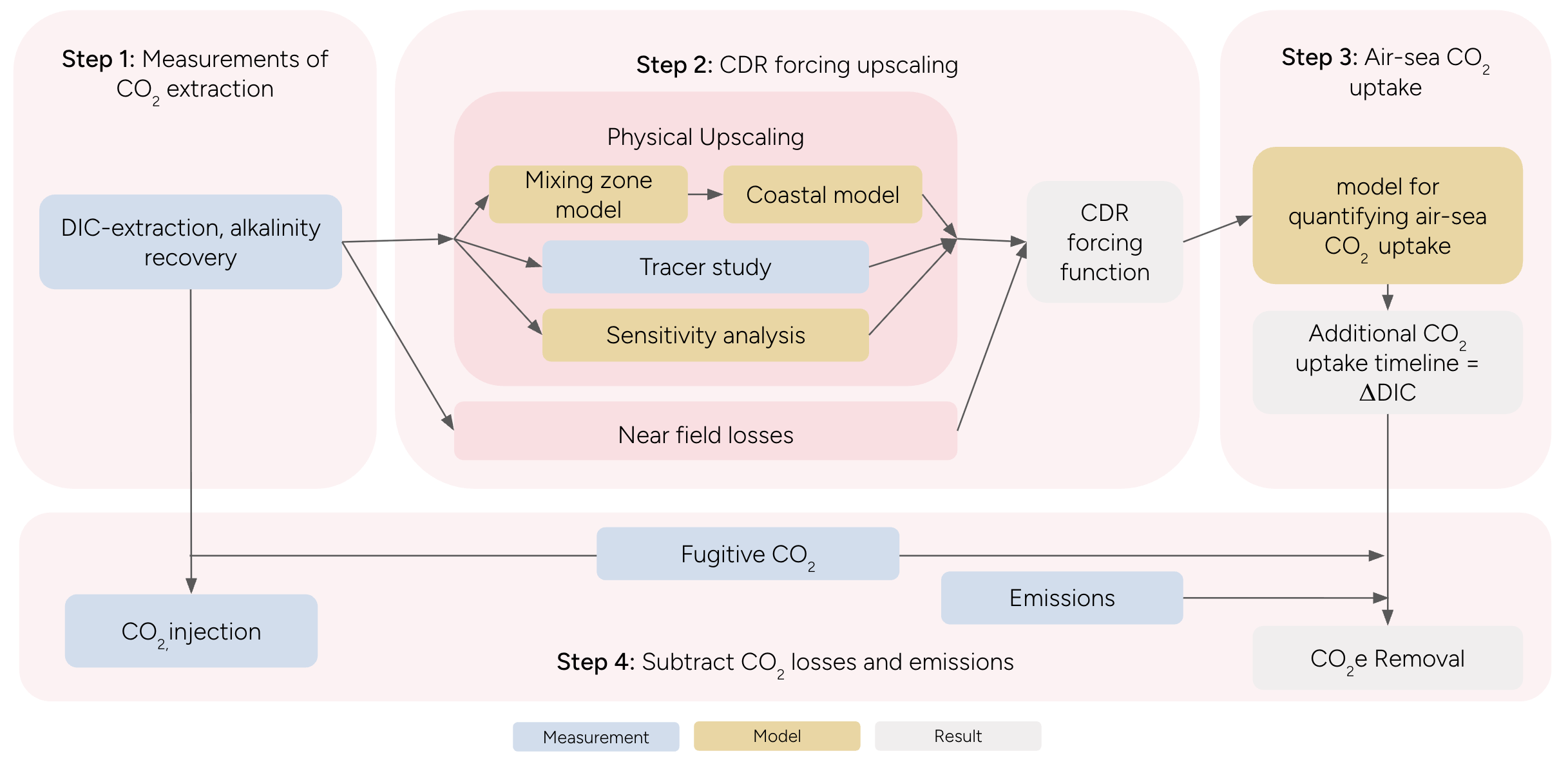
Figure A3-1 Example of quantification options described in Section 7.4.1.
Footnotes
-
Eisaman, M. D. (2024). Pathways for marine carbon dioxide removal using electrochemical acid-base generation. Frontiers in Climate, 6, 1349604, https://www.frontiersin.org/journals/climate/articles/10.3389/fclim.2024.1349604 ↩
-
National Academies of Sciences, Engineering, and Medicine. (2022). A Research Strategy for Ocean-based Carbon Dioxide Removal and Sequestration. Washington, DC: The National Academies Press. https://doi.org/10.17226/26278. ↩ ↩2 ↩3 ↩4
-
Rocky Mountain Institute. The Applied Innovation Roadmap for CDR. https://rmi.org/insight/the-applied-innovation-roadmap-for-cdr/ ↩ ↩2
-
Cross, J.N., Sweeney, C., Jewett, E.B., Feely, R.A., McElhany, P., Carter, B., Stein, T., Kitch, G.D., and Gledhill, D.K. (2023). Strategy for NOAA Carbon Dioxide Removal Research: A white paper documenting a potential NOAA CDR Science Strategy as an element of NOAA’s Climate Interventions Portfolio. NOAA Special Report. https://sciencecouncil.noaa.gov/wp-content/uploads/2023/06/mCDR-glossy-final.pdf ↩ ↩2 ↩3
-
de Lannoy, C. F., Eisaman, M. D., Jose, A., Karnitz, S. D., DeVaul, R. W., Hannun, K., & Rivest, J. L. (2018). Indirect ocean capture of atmospheric CO2: Part I. Prototype of a negative emissions technology. International journal of greenhouse gas control, 70, 243-253. https://doi.org/10.1016/j.ijggc.2017.10.007 ↩
-
Marine Carbon Dioxide Removal Field Trial Database. Ocean Visions. Retrieved May 7, 2025 from https://oceanvisions.org/mcdr-field-trials/. ↩
-
Methodology for assessing the quality of carbon Credits. Version 3.0 (2022). World Wildlife Fund, Environmental Defense Fund and Oeko-Institute Report. https://carboncreditquality.org/download/Methodology/CCQI%20Methodology%20-%20Version%203.0.pdf ↩
-
Oschlies, A., Stevenson, A., Bach, L. T., Fennel, K., Rickaby, R. E. M., Satterfield, T., Webb, R., and Gattuso, J.-P. (2023). Guide to Best Practices in Ocean Alkalinity Enhancement Research, State of the Planet, 2-oae2023, https://doi.org/10.5194/sp-2-oae2023. ↩
-
Wilkinson, M., Dumontier, M., Aalbersberg, I. et al. (2016). The FAIR Guiding Principles for scientific data management and stewardship. Scientific Data 3, 160018. https://doi.org/10.1038/sdata.2016.18 ↩ ↩2
-
Steenkamp, R. and Webb, R. (2023) Legal considerations relevant to research on ocean alkalinity enhancement. State of the Planet. https://doi.org/10.5194/sp-2-oae2023-10-2023 ↩ ↩2
-
Satterfield et al. (2023) Social considerations and best practices to apply to engaging publics on ocean alkalinity enhancement. State of the Planet. https://doi.org/10.5194/sp-2-oae2023-11-2023 ↩
-
Webb et al. (2021) Removing Carbon Dioxide Through Ocean Alkalinity Enhancement and Seaweed Cultivation: Legal Challenges and Opportunities, Sabin Center for Climate Change Law [working draft] https://papers.ssrn.com/sol3/papers.cfm?abstract_id=3800494 ↩
-
Permitting for mCDR and mSRM. United States Environmental Protection Agency. Retrieved May 17, 2024, from https://www.epa.gov/ocean-dumping/permitting-mcdr-and-msrm ↩
-
Albright, R., Caldeira, L., Hosfelt, J. et al. (2016). Reversal of ocean acidification enhances net coral reef calcification. Nature 531, 362–365. https://doi.org/10.1038/nature17155 ↩
-
Missimer, T., Maliva, R. (2018). Environmental issues in seawater reverse osmosis desalination: Intakes and outfalls. Desalination. https://doi.org/10.1016/j.desal.2017.07.012 ↩
-
Hogan, T. W. (2015). Impingement and entrainment at SWRO Desalination Facility intakes. Environmental Science and Engineering. https://doi.org/10.1007/978-3-319-13203-7_4 ↩
-
IPCC, 2023: Climate Change 2023: Synthesis Report. Contribution of Working Groups I, II and III to the Sixth Assessment Report of the Intergovernmental Panel on Climate Change [Core Writing Team, H. Lee and J. Romero (eds.)]. IPCC. doi: 10.59327/IPCC/AR6-9789291691647. ↩
-
Fennel, K., Long, M. C., Algar, C., et al. (2023) Modelling considerations for research on ocean alkalinity enhancement (OAE). State of the Planet 2-oae2023, 9, https://doi.org/10.5194/sp-2-oae2023-9-2023 ↩
-
Pytkowicz (1965). Calcium Carbonate Precipitation in the Ocean. Limnology and Oceanography. https://doi.org/10.4319/lo.1965.10.2.0220 ↩
-
Moras, C. A., Bach, L. T., Cyronak, T., et. al. (2022). Ocean alkalinity enhancement – avoiding runaway CaCO3 precipitation during quick and hydrated lime dissolution, Biogeosciences, 19, 3537–3557, https://doi.org/10.5194/bg-19-3537-2022 ↩
-
Turchyn AV, Bradbury HJ, Walker K and Sun X. (2021) Controls on the Precipitation of Carbonate Minerals Within Marine Sediments. Frontiers in Earth Science 9:618311. doi: 10.3389/feart.2021.618311 ↩
-
Renforth, P., and G. Henderson. (2017). Assessing ocean alkalinity for carbon sequestration, Reviews of Geophysics, 55, 636–674, doi:10.1002/2016RG000533 ↩ ↩2
-
Morse, J. W., He, S. (1993). Influences of T, S and P CO₂ on the pseudo-homogeneous precipitation of CaCO3 from seawater: implications for whiting formation. Marine Chemistry. https://doi.org/10.1016/0304-4203(93)90261-L ↩
-
Wurgaft, E., Wang, Z. A., Churchill, J. H., Dellapenna, T., Song, S., Du, J., et al. (2021). Particle triggered reactions as an important mechanism of alkalinity and inorganic carbon removal in river plumes. Geophysical Research Letters, 48, e2021GL093178. https://doi.org/10.1029/2021GL093178 ↩
-
Ringham, M., Hirtle, N., Shaw, C., Lu, X., Herndon, J., Carter, B., and Eisaman, M. (2024). A comprehensive assessment of electrochemical ocean alkalinity enhancement in seawater: kinetics, efficiency, and precipitation thresholds, EGUsphere [preprint], https://doi.org/10.5194/egusphere-2024-108 ↩ ↩2
-
Schulz, K. G., Bach, L. T., and Dickson, A. G. (2023). Seawater carbonate chemistry considerations for ocean alkalinity enhancement research: theory, measurements, and calculations, in: Guide to Best Practices in Ocean Alkalinity Enhancement Research. Copernicus Publications, State Planet, 2-oae2023, 2, https://doi.org/10.5194/sp-2-oae2023-2-2023 https://doi.org/10.1038/nature17155 ↩
-
Moras, C. A., Bach, L. T., Cyronak, T., Joannes-Boyau, R., and Schulz, K. G. (2022) Ocean alkalinity enhancement – avoiding runaway CaCO3 precipitation during quick and hydrated lime dissolution, Biogeosciences, 19, 3537–3557, https://doi.org/10.5194/bg-19-3537-2022. ↩ ↩2
-
Iglesias-Rodríguez, M. D., Rickaby, R. E. M., Singh, A., and Gately, J. A. (2023). Laboratory experiments in ocean alkalinity enhancement research, in: Guide to Best Practices in Ocean Alkalinity Enhancement Research, Copernicus Publications, State Planet, 2-oae2023, 5, https://doi.org/10.5194/sp-2-oae2023-5-2023. ↩
-
He and Tyka (2023) Limits and CO2 equilibration of near-coast alkalinity enhancement. Biogeosciences, 20, 27–43. https://doi.org/10.5194/bg-20-27-2023 ↩
-
Hartmann, J., Suitner, N., Lim, C., Schneider, J., Marín-Samper, L., Arístegui, J., ... & Riebesell, U. (2022). Stability of alkalinity in ocean alkalinity enhancement (OAE) approaches–consequences for durability of CO 2 storage. Biogeosciences Discussions, 2022, 1-29. https://doi.org/10.5194/bg-20-781-2023 ↩
-
Jokiel, P. L. (2011). The reef coral two compartment proton flux model: A new approach relating tissue-level physiological processes to gross corallum morphology. Journal of Experimental Marine Biology and Ecology, 409(1–2), 1–12. https://doi.org/10.1016/j.jembe.2011.10.008 ↩
-
Bach, L. T. (2015). Reconsidering the role of carbonate ion concentration in calcification by marine organisms. Biogeosciences, 12(16), 4939-4951. ↩
-
Monteiro, F. M., Bach, L. T., Brownlee, C., Bown, P., Rickaby, R. E. M., Poulton, A. J., et al. (2016). Why marine phytoplankton calcify (supplement). Sci. Adv. 2:e1501822. doi: 10.1126/sciadv.1501822 ↩
-
Bach, L.T., Gill, S.J., Rickaby R.E.M., et. al. (2019) CO₂ Removal With Enhanced Weathering and Ocean Alkalinity Enhancement: Potential Risks and Co-benefits for Marine Pelagic Ecosystems. Frontiers in Climate. 1:7. doi: 10.3389/fclim.2019.00007 ↩ ↩2
-
Gately, J..A., Kim, S.M., Jin, B., et al. (2023). Coccolithophores and diatoms resilient to ocean alkalinity enhancement: A glimpse of hope?. Science Advances 9, eadg6066. DOI:10.1126/sciadv.adg6066 ↩ ↩2
-
Subhas AV, Marx L, Reynolds S., et. al. (2022). Microbial ecosystem responses to alkalinity enhancement in the North Atlantic Subtropical Gyre. Frontiers in Climate. 4:784997. doi: 10.3389/fclim.2022.784997 ↩
-
Hay, B. J. (1988). Sediment accumulation in the central western part of the Black Sea over the last 5100 years. Paleoocenography 3, 491–508. doi:10.1029/PA003i004p00491 ↩
-
Kopelevich, O., Burenkov, V., Sheberstov, S., Vazyulya, S., Kravchishina, M., Pautova, L., et al. (2014). Satellite monitoring of coccolithophore blooms in the Black Sea from ocean color data. Remote Sens. Environ. 146, 113–123. doi: 10.1016/j.rse.2013.09.009 ↩
-
Bednaršek, N., van de Mortel, H., Pelletier, G., García-Reyes, M., Feely, R. A., & Dickson, A. G. (2025). Assessment framework to predict sensitivity of marine calcifiers to ocean alkalinity enhancement–identification of biological thresholds and importance of precautionary principle. Biogeosciences, 22(2), 473-498. https://doi.org/10.5194/bg-22-473-2025. ↩
-
Bach, L. T. (2023) The additionality problem of Ocean Alkalinity Enhancement. Biogeosciences 21, 261–277. https://bg.copernicus.org/articles/21/261/2024/ ↩
-
Gutiérrez-Loza, L., Nilsson, E., Wallin, M. B., Sahlée, E., & Rutgersson, A. (2022). On physical mechanisms controlling air-sea CO 2 exchange. Biogeosciences Discussions, 2022, 1-24. https://doi.org/10.5194/bg-19-5645-2022 ↩
-
Adefila, K., Yan, Y., Sun, L., & Wang, T. (2017). Flow measurement of wet CO2 using an averaging pitot tube and coriolis mass flowmeters. International Journal of Greenhouse Gas Control, 63, 289–295. https://doi.org/10.1016/J.IJGGC.2017.06.005 ↩
-
Schaap, A., Papadimitriou, S., Mawji, E., Walk, J., Hammermeister, E., Mowlem, M., & Loucaides, S. (2025). Autonomous sensor for in situ measurements of total alkalinity in the ocean. ACS Sensors. https://doi.org/10.1021/acssensors.4c02349 ↩
-
Raimondi, L., Matthews, J. B. R., Atamanchuk, D., Azetsu-Scott, K., Wallace, D. W. R. (2019) The internal consistency of the marine carbon dioxide system for high latitude shipboard and in situ monitoring. Marine Chemistry, 213, 49-70, doi:10.1016/j.marchem.2019.03.001 ↩
-
Mu, L., Palter, J. B., & Wang, H. (2023). Considerations for hypothetical carbon dioxide removal via alkalinity addition in the Amazon River watershed. Biogeosciences, 20(10), 1963–1977. https://doi.org/10.5194/bg-20-1963-2023 ↩
-
United States Environmental Protection Agency: Compilation of EPA Mixing Zone Documents. Retrieved May 29, 2024, from https://www.epa.gov/sites/default/files/2018-10/documents/compilation-epa-mixingzone-documents.pdf ↩
-
Jiang, L.-Q., Subhas, A. V., Basso, D., Fennel, K., and Gattuso, J.-P. (2023) Data reporting and sharing for ocean alkalinity enhancement research. State of the Planet 2-oae2023, 13, https://doi.org/10.5194/sp-2-oae2023-13-2023 ↩
-
National Oceanic and Atmospheric Administration , (2023). OA Metadata Template (Version 2.0). National Centers for Environmental Information. https://www.ncei.noaa.gov/access/ocean-carbon-acidification-data-system/oa-metadata-template/ ↩
-
Middelburg, J. J., Soetaert, K., and Hagens, M. (2020) Ocean Alkalinity, Buffering and Biogeochemical Processes. Reviews of Geophysics, 58, https://doi.org/10.1029/2019RG000681 ↩
-
Dickson, A. G., An exact definition of total alkalinity and a procedure for the estimation of alkalinity and total inorganic carbon from titration data. Deep Sea Research Part A. Oceanographic Research Papers, 28 (6), 609-623. https://doi.org/10.1016/0198-0149(81)90121-7 ↩
-
Mario, G. M., Millero, F. J., Camões, M.F., Spitzer, P., Feistel, R., and Chen, C.-T.A. (2011) pH of seawater. Marine Chemistry, 126(1-4), 89-96. https://doi.org/10.1016/j.marchem.2011.04.002 ↩
-
Pimenta, A. R., and Grear, J. S. (2018). Guidelines for Measuring Changes in Seawater pH and Associated Carbonate Chemistry in Coastal Environments of the Eastern United States. United States Environmental Protection Agency. Retrieved July 1, 2024, from https://www.goa-on.org/documents/resources/east-us-measuring_seawater_ph_changes-guide.pdf ↩
-
Jiang, L., Pierrot, D., Wanninkhof, R. et al. (2023). Best Practice Data Standards for Discrete Chemical Oceanographic Observations. Frontiers in Marine Science. https://www.frontiersin.org/articles/10.3389/fmars.2021.705638/full ↩
-
Schulz, K. G., Bach, L. T., and Dickson, A. G.: Seawater carbonate chemistry considerations for ocean alkalinity enhancement research: theory, measurements, and calculations. State of the Planet, 2-oae2023, 2, https://doi.org/10.5194/sp-2-oae2023-2-2023. ↩
-
Bushnell M, Waldmann C, Seitz S, et al. (2019). Quality Assurance of Oceanographic Observations: Standards and Guidance Adopted by an International Partnership. Frontiers in Marine Science, 6:706 https://www.frontiersin.org/articles/10.3389/fmars.2019.00706/full ↩
-
Thomson, R. and Emery, W. (2014) Data Analysis Methods in Physical Oceanography. https://www.sciencedirect.com/book/9780123877826/data-analysis-methods-in-physical-oceanography#book-description ↩
-
Science and Ecosystem Support Divison (2017). Dye Tracer Measurements Operating Procedure. U.S. Environmental Protection Agency. https://www.epa.gov/sites/default/files/2017-07/documents/dye_tracer_measurements514_af.r2.pdf ↩
-
Wilson, J. F., Cobb, E. D., & Kilpatrick, F. A. (1986). Fluorometric procedures for dye tracing. In Techniques of Water-Resources Investigations (03-A12). Dept. of the Interior, U.S. Geological Survey; For sale by the Books and Open-File Reports Section, U.S. Geological Survey,. https://doi.org/10.3133/twri03A12 ↩
-
Jirka GH, Harleman DRF. (1979). Stability and mixing of a vertical plane buoyant jet in confined depth. Journal of Fluid Mechanics. 1979;94(2):275-304. doi:10.1017/S0022112079001038 ↩
Contributors

Jennifer Yin, Ph.D.

Jing He, Ph.D.

Sophie Gill, Ph.D.

Kevin Sutherland, Ph.D.

Emma Marsland

Jasmin Kazazi
Isometric
Direct Ocean Capture and Storage © 2025 Isometric HQ Ltd is licensed under CC BY-NC-ND 4.0